Tutorial 5, Week 10 Solutions
Q1
(a)
\[\tilde{f}(x) = \frac{1}{2} \exp(-|x|) \quad \forall\,x \in \mathbb{R}\]
\[\begin{align*} \tilde{F}(x) &= \int_{-\infty}^x \tilde{f}(z)\,dz \\ &= \begin{cases} \displaystyle \frac{1}{2} \int_{-\infty}^x \exp(z) \,dz & \text{if }x \le 0 \\ \displaystyle \frac{1}{2} + \frac{1}{2} \int_0^x \exp(-z) \,dz & \text{if }x > 0 \end{cases} \end{align*}\]
The first integral is trivially \(e^x\). For the second integral, you can either use a simple symmetry argument, or, to plough through the calculus directly we could use the substitution \(u = -z \implies du = -dz\) and limits \(u = -0 = 0\) to \(u = -x\),
\[\int_0^x \exp(-z) \,dz = -\int_0^{-x} \exp(u) \,du = -e^u \Big|_0^{-x} = 1-e^{-x}\]
Therefore,
\[ \tilde{F}(x) = \begin{cases} \displaystyle \frac{e^x}{2} & \text{if }x \le 0 \\ \displaystyle 1 - \frac{e^{-x}}{2} & \text{if }x > 0 \end{cases} \]
The generalised inverse is thus,
\[ \tilde{F}^{-1}(u) = \begin{cases} \displaystyle \log(2u) & \text{if }u \le \frac{1}{2} \\ \displaystyle -\log(2-2u) & \text{if }u > \frac{1}{2} \end{cases} \]
Hence, to inverse sample a standard Laplace random variable we would generate \(U \sim \text{Unif}(0,1)\) and compute \(\tilde{F}^{-1}(U)\) per above.
(b)
We require \(c < \infty\) such that
\[\frac{1}{\sqrt{2 \pi}} \exp\left(-\frac{x^2}{2}\right) \le \frac{c}{2} \exp(-|x|) \quad \forall\ x \in \mathbb{R}\]
Both pdfs are symmetric about zero, so this is equivalent to:
\[\frac{1}{\sqrt{2 \pi}} \exp\left(-\frac{x^2}{2}\right) \le \frac{c}{2} \exp(-x) \quad \forall\ x \in [0,\infty)\]
In other words, we require:
\[c = \sup_{x \in [0,\infty)} \sqrt{\frac{2}{\pi}} \exp\left( -\frac{x^2}{2} + x \right)\]
As \(x\to\infty\), the \(-x^2/2\) dominates the \(+x\), so the exponential term tends to zero and we can see there is no problem in the tail.
Now,
\[\begin{align*} \frac{d}{dx} &= \sqrt{\frac{2}{\pi}} (1-x) \exp\left( -\frac{x^2}{2} + x \right) & \text{Simple chain rule application} \\ \frac{d^2}{dx^2} &= \sqrt{\frac{2}{\pi}} x (x-2) \exp\left( -\frac{x^2}{2} + x \right) & \text{Product and chain rules} \end{align*}\]
By inspection, \(d/dx = 0 \iff x = 1\) and at this point \(d^2/dx^2 < 0\) confirming this is a maximum. Hence,
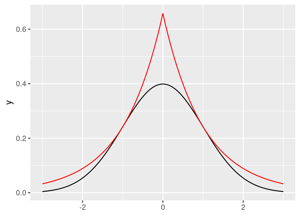
\[c = \sqrt{\frac{2}{\pi}} \exp\left( \frac{1}{2} \right) \approx 1.3155\]
The following graph shows the standard Laplace distribution scaled by \(c\) in red, with the standard normal in black, confirming that \(c\) satisfies the inequality.
(c)
- Set \(a \leftarrow \texttt{FALSE}\)
- While \(a\) is \(\texttt{FALSE}\),
- Generate \(U_1 \sim \text{Unif}(0,1)\)
- Compute \[X = \begin{cases} \displaystyle \log(2U_1) & \text{if }U_1 \le \frac{1}{2} \\ \displaystyle -\log(2-2U_1) & \text{if }U_1 > \frac{1}{2} \end{cases}\] which generates a proposal from the standard Laplace distribution.
- Generate \(U_2 \sim \text{Unif}(0,1)\)
- If \[U_2 \le \frac{1}{1.3155}\sqrt{\frac{2}{\pi}} \exp\left(-\frac{X^2}{2} + |X|\right)\] then set \(a \leftarrow \texttt{TRUE}\)
- Return \(X\) as a sample from \(\text{N}(0,1)\).
(d)
By Lemma 5.1, the expected number of iterations of the rejection sampler required to produce a sample is given by \(c\), so since here \(c\approx1.3155 < 1.521\) we would favour using the standard Laplace distribution as a proposal. The Cauchy proposal would require \(\left( 1.521/1.3155 - 1 \right)\% \approx 15.6\%\) more iterations to produce any given number of standard Normal simulations.
Q2
(a)
By kindergarden rules of probability,
\[\begin{align*} \mathbb{P}(X \le x \given a \le X \le b) &= \frac{\mathbb{P}(a \le X \le b \cap X \le x)}{\mathbb{P}(a \le X \le b)} \\[5pt] &= \frac{\mathbb{P}(a \le X \le b \cap X \le x)}{F(b) - F(a)} \end{align*}\]
Taking the numerator separately,
\[\begin{align*} \mathbb{P}(a \le X \le b \cap X \le x) &= \begin{cases} 0 & \text{if } x < a \\[5pt] \mathbb{P}(a \le X \le x) & \text{if } a \le x \le b \\[5pt] \mathbb{P}(a \le X \le b) & \text{if } x > b \end{cases} \\[10pt] &= \begin{cases} 0 & \text{if } x < a \\[5pt] F(x) - F(a) & \text{if } a \le x \le b \\[5pt] F(b) - F(a) & \text{if } x > b \end{cases} \end{align*}\]
Therefore,
\[ \mathbb{P}(X \le x \given a \le X \le b) = \begin{cases} 0 & \text{if } x < a \\[5pt] \displaystyle \frac{F(x) - F(a)}{F(b)- F(a)} & \text{if } a \le x \le b \\[5pt] 1 & \text{if } x > b \end{cases} \]
(b)
We simply want to find the generalised inverse of the cdf we just derived. So if \(U \sim \text{Unif}(0,1)\), then we solve for \(X\) in:
\[\begin{align*} U &= \frac{F(X) - F(a)}{F(b)- F(a)} \\[5pt] \implies F(X) &= U \big( F(b)- F(a) \big) + F(a) \\[5pt] \implies X &= F^{-1}\Big( U \big( F(b)- F(a) \big) + F(a) \Big) \end{align*}\]
(c)
For an Exponential distribution, \(F(x) = 1-e^{-\lambda x}\) and therefore \(F^{-1}(u) = -\lambda^{-1} \log(1-u)\).
Truncating to \(X \in [1, \infty) \implies a = 1, b = \infty\), thus \(F(a) = 1-e^{-\lambda}, F(b) = 1\) and so the inverse sampler is:
\[\begin{align*} X &= F^{-1}\Big( U \big( F(b)- F(a) \big) + F(a) \Big) \\ &= F^{-1}\Big( U \big( 1 - (1-e^{-\lambda}) \big) + (1-e^{-\lambda}) \Big) \\ &= F^{-1}\Big( e^{-\lambda} \big( U - 1 \big) + 1 \Big) \\ &= -\lambda^{-1} \log\Big( 1 - \big( e^{-\lambda} \big( U - 1 \big) + 1 \big) \Big) \\ &= -\lambda^{-1} \log\Big( e^{-\lambda} \big( 1 - U \big) \Big) \\ &= 1 - \lambda^{-1} \log\big( 1 - U \big) \\ \end{align*}\]
(d)
Notice that the inverse sampler for the Exponential distribution truncated to \([1, \infty)\) is simply \(1 + \big(- \lambda^{-1} \log( 1 - U )\big)\) … in other words, inverse sample a standard Exponential and add 1!
This agrees with the well-known memoryless property of the Exponential distribution.
Note: obviously for other distributions it will not be so simple, this is a very special property of Exponential random variables.