$$ \require{cancel} \newcommand{\given}{ \,|\, } \renewcommand{\vec}[1]{\mathbf{#1}} \newcommand{\vecg}[1]{\boldsymbol{#1}} \newcommand{\mat}[1]{\mathbf{#1}} \newcommand{\bbone}{\unicode{x1D7D9}} $$

Lab 3: Data frame loading/exploring

This lab is intentionally slightly shorter, because Lab 2 was quite long … 🧑‍💻 So make sure to finish Lab 2 before continuing with this lab!

Don’t feel the need to rush, it’s better to understand everything solidly and be a little behind — and you are welcome to ask questions about any of the labs throughout the term! 🙋‍♀️

Wine quality 🍷

Real world data rarely involves only one variable. Therefore, statisticians usually collect data together into design matrices, as we discussed in the lecture last week.

Exercise 5.20 Manually create a small data frame containing the design matrix below, and store it in the variable X. Use this to compute the mean of each variable.

sugars	pH	alcohol
1.9	3.51	9.4
2.6	3.20	9.8
2.3	3.26	9.8
1.9	3.16	9.8

Click for solution

## SOLUTION

X <- data.frame(sugars = c(1.9, 2.6, 2.3, 1.9),
                pH = c(3.51, 3.20, 3.26, 3.16),
                alcohol = c(9.4, 9.8, 9.8, 9.8))

# Either of the following could get the means
colMeans(X)

 sugars      pH alcohol 
 2.1750  3.2825  9.7000 

summary(X)

     sugars            pH           alcohol   
 Min.   :1.900   Min.   :3.160   Min.   :9.4  
 1st Qu.:1.900   1st Qu.:3.190   1st Qu.:9.7  
 Median :2.100   Median :3.230   Median :9.8  
 Mean   :2.175   Mean   :3.283   Mean   :9.7  
 3rd Qu.:2.375   3rd Qu.:3.322   3rd Qu.:9.8  
 Max.   :2.600   Max.   :3.510   Max.   :9.8  

This is in fact just a snippet of data from a large set of data collected on different wines. Visit the following web page to see more details about the available data: https://archive.ics.uci.edu/ml/datasets/Wine+Quality This website is the “UCI machine learning repository” which contains a lot of data used to benchmark the performance of machine learning algorithms and can be interesting to explore.

By clicking on the blue “Download” button near the top right of the page, you will be able to download a .zip file containing two CSV files with data on red wine and white wine (and another text file with information about the data).

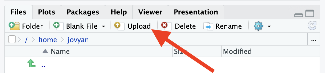
Exercise 5.21 Download and unzip the file to find the two data files winequality-red.csv and winequality-white.csv. If you are using the Github Codespaces server, upload these files to the server using the “Upload” button in the “Files” pane; if you’re using your own computer or AppsAnywhere, there is no need to upload (and there will be no upload button). If you are using an iPad to access Github Codespaces, you might not be able to unzip the downloaded file: don’t worry, just upload the .zip directly and RStudio will automatically unzip the files for you.

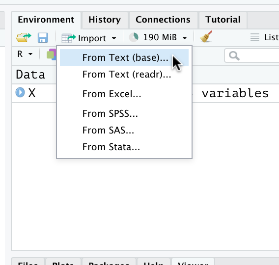
Exercise 5.22 Using the RStudio “Import” button in the “Environment” tab, import the first data set into a variable called wq.red and the second into a variable called wq.white.

Click for solution

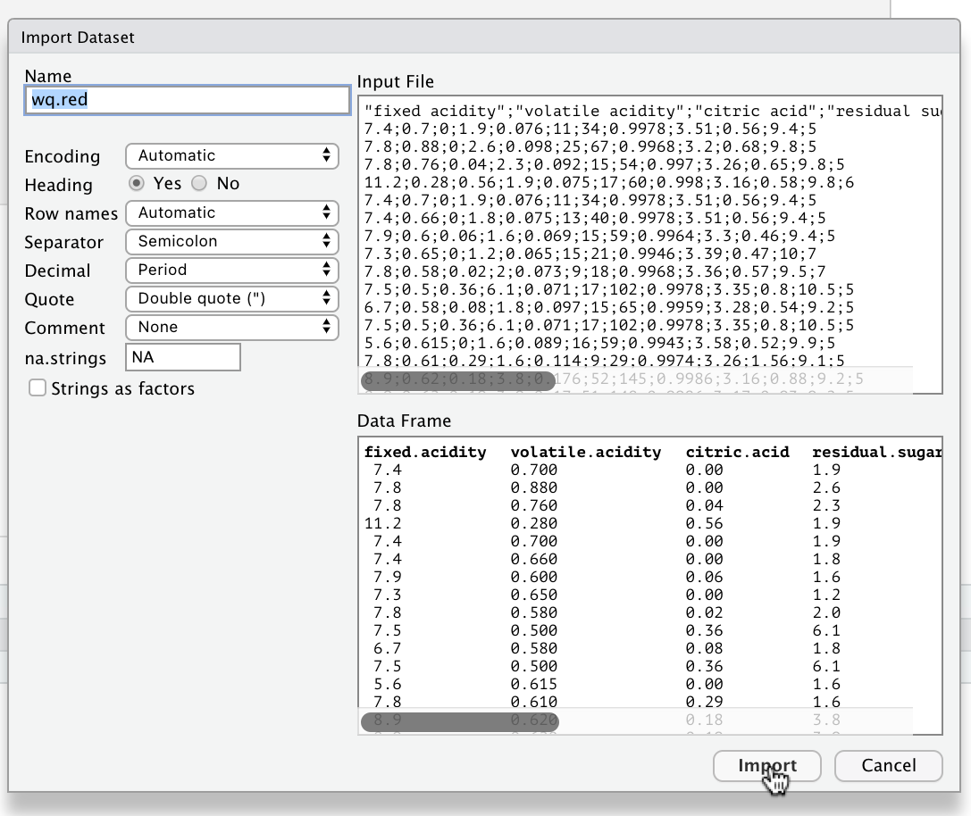
Step 1: Step 2: (you’ll need to locate the file wherever you downloaded it) Step 3:

NOTE 1: you need to update the name of the variable in the top left to wq.red or wq.white per the question.

NOTE 2: look carefully and you will see that the input file is actually separated not by commas, but by semi colons ;. This is an example of the kind of oddity you will encounter with real world data. Fortunately RStudio detected this and if you look closely the drop down box option for “Separator” was automatically changed from comma to semi colon!

This will then automatically run something like the following in your console (with the correct path for your system to the file):

wq.red <- read.csv("winequality-red.csv", sep=";")
View(wq.red)

NOTE: you need to repeat these steps to load the white wine data into wq.white.

It is believed that the sulphate levels play an important role in the perceived quality of a red wine 🍷. Red wines with elevated sulphate levels are thought to taste a little better.

R has some very nice plotting capabilities available in add-on packages which we’ll look at in lectures soon. It also has some quick and easy (but slightly less visually appealing) plotting capabilities built-in. We can produce a scatter plot very easily by using the plot() function. You can either:

• pass two vectors of the same length as the first two arguments, it will plot the first vector as the \(x\) coordinates and the second as the \(y\) coordinates; or
• pass a data frame with two columns and it will plot the first variable on the \(x\) axis and the second on the \(y\).

Exercise 5.23 Identify which variables in wq.red contain the sulphates and quality variables and therefore plot quality (y-axis) against sulphates (x-axis).

Click for solution

# Can be solved a few ways: try to understand all of them!

## SOLUTION 1
names(wq.red)
# from the above we see they are variables 9, 10 and 12, so:
plot(wq.red[,c(10,12)])

## SOLUTION 2
# we could directly pull the variables as vectors and pass two arguments
plot(wq.red$sulphates, wq.red$quality)

## SOLUTION 3
# we can in fact pass the vector of names as the columns we want to select directly
# this is similar to solution 1 but using the names not numbers
plot(wq.red[,c("sulphates","quality")])

The relationship is clearly weak if it is there!

Exercise 5.24 Let’s split the dataset into two parts: the half with lowest sulphates and the half with highest sulphates.

1. Calculate the median sulphate level in the red wines;
2. Subset the rows of wq.red to select all red wines with sulphate level less than or equal to the median and store them in a variable called low.s
3. Subset the rows of wq.red to select all red wines with sulphate level greater than the median and store them in a variable called high.s

Click for solution

## SOLUTION

median(wq.red$sulphates)

[1] 0.62

low.s <- wq.red[wq.red$sulphates <= median(wq.red$sulphates),]
high.s <- wq.red[wq.red$sulphates > median(wq.red$sulphates),]

Exercise 5.25 By using code you saw in the lecture on Bootstrap, plot the empirical cdf of the low sulphate wine qualities.

Hint: see the code box following Theorem 3.1.

Click for solution

## SOLUTION

low.ecdf <- ecdf(low.s$quality)
plot(low.ecdf)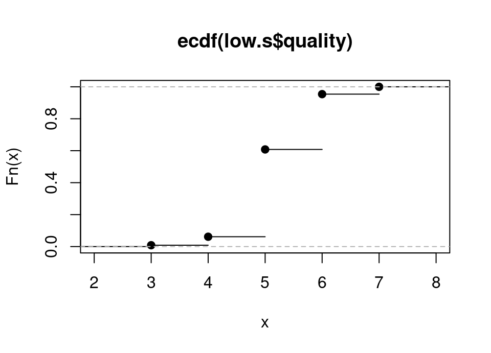

Every time you call the plot() function, it causes an entirely new plot to be created. Sometimes, we want to build up the plot we require by layering multiple plots, rather than always starting from a clean slate. To add more lines to a plot, we use lines(), and otherwise pass exactly what we would have passed to the plot() function … the difference is that the content will be added to the existing plot, rather than triggering a fresh clean plot.

Exercise 5.26 Add to the plot of the empirical cdf of the low sulphate wine qualities an overlay with the empirical cdf of the high sulphate wine qualities.

Hint: if you also provide the named argument col="red" when calling the lines() function it will be easier to distinguish which ecdf is which.

Click for solution

## SOLUTION

# Running the previous plot ...
plot(low.ecdf)
# ... followed immediately by lines will add to it rather than making a new
# plot
high.ecdf <- ecdf(high.s$quality)
lines(high.ecdf, col = "red")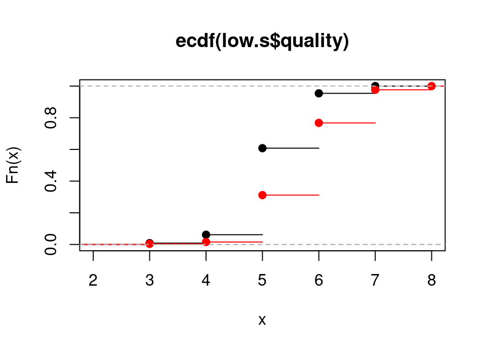

Exercise 5.27 The ecdf() function is interesting, because what it returns is actually a function! This function evaluates \(\hat{F}(x)\). Read the “Details” section of the help file to confirm that the definition matches lectures.

1. Recall from lectures that str() is useful for examining unknown objects in R. Use str() to confirm that the two ecdfs you computed for low/high sulphate qualities above are indeed functions.
2. Let \(Q_\ell\) and \(Q_h\) be the random variables representing wine quality for low and high sulphate wines as defined before. Use the functions returned by ecdf() to estimate \(\mathbb{P}(Q_\ell \le 5)\) and \(\mathbb{P}(Q_h \ge 7)\)

Click for solution

## SOLUTION

# Examine the ecdf objects we computed earlier and notice they are functions
str(low.ecdf)

function (v)  
 - attr(*, "class")= chr [1:3] "ecdf" "stepfun" "function"
 - attr(*, "call")= language ecdf(low.s$quality)

str(high.ecdf)

function (v)  
 - attr(*, "class")= chr [1:3] "ecdf" "stepfun" "function"
 - attr(*, "call")= language ecdf(high.s$quality)

# Use these to compute the required probabilities
low.ecdf(5)

[1] 0.6079614

1-high.ecdf(6)

[1] 0.2324675

You could see from the various plots above that the quality values are on an integer scale and therefore clearly not Normal. However, we have a very large sample so the mean will already be entering the asymptotic regime where the central limit theorem applies and the sampling distribution of the mean will be approximately Normal. R lets us really easily do Stats 1 style confidence intervals and t-tests using the t.test() function: you just supply it a vector of numbers and it will by default conduct a hypothesis test that the mean is zero and also find the confidence interval for the mean (look at the help file ?t.test if you want to test a non-zero mean).

Exercise 5.28 Compute the confidence interval for the mean wine quality of the top 50% of sulphate content red wines and also separately for the bottom 50% of sulphate content wines.

Do the confidence intervals for mean quality in each group overlap, or is there evidence that high/low sulphate wines have on average higher/lower mean quality?

Click for solution

## SOLUTION

t.test(low.s$quality)

    One Sample t-test

data:  low.s$quality
t = 222.7, df = 828, p-value < 2.2e-16
alternative hypothesis: true mean is not equal to 0
95 percent confidence interval:
 5.320602 5.415224
sample estimates:
mean of x 
 5.367913 

Reading the output of the t-test shows the 95% confidence interval for mean wine quality among low sulphate wines is (5.32, 5.42).

t.test(high.s$quality)

    One Sample t-test

data:  high.s$quality
t = 200, df = 769, p-value < 2.2e-16
alternative hypothesis: true mean is not equal to 0
95 percent confidence interval:
 5.866522 5.982828
sample estimates:
mean of x 
 5.924675 

Reading the output of the t-test shows the 95% confidence interval for mean wine quality among high sulphate wines is (5.87, 5.98).

The two intervals do no overlap, so there is evidence to suggest high sulphate content wines do have a higher mean quality than low sulphate wines.

It is suspected that although high sulphate content wines are on average higher quality, they are of less consistent quality: statistically this translates to having a higher variance (or standard deviation).

Exercise 5.29 We can use Bootstrap to estimate the confidence interval of the standard deviation in wine quality for high and low sulphate red wines, even though we don’t know the sampling distribution of the standard deviation. Perform this analysis to estimate the standard error of the standard deviation of quality in high and low sulphate wines.

Can you conclude that there is a difference in consistency of quality between sulphate levels?

Click for solution

## SOLUTION

high.s.sd <- rep(0, 1000)
low.s.sd <- rep(0, 1000)
for(i in 1:1000) {
  high.s.star <- sample(high.s$quality, replace = TRUE)
  high.s.sd[i] <- sd(high.s.star)
  
  low.s.star <- sample(low.s$quality, replace = TRUE)
  low.s.sd[i] <- sd(low.s.star)
}

# Estimator of the high sulphate wine quality standard deviation
sd(high.s$quality)

[1] 0.8220239

# Bootstrap estimate of the standard error in our standard deviation
sd(high.s.sd)

[1] 0.02038673

# Estimator of the low sulphate wine quality standard deviation
sd(low.s$quality)

[1] 0.6939929

# Bootstrap estimate of the standard error in our standard deviation
sd(low.s.sd)

[1] 0.01928192

Remember, our actual estimator is just the statistic of interest applied to the original data, so we have the estimator of the standard deviation of high and low sulphate wines is about 0.822 and 0.693 respectively. Then we use the Bootstrap simulations to find the standard error in the estimator of the standard deviation of high and low sulphate wines (that’s quite a mouthful!) is about 0.02 in both cases … you will get slightly varying answers due to random sampling.

Consequently we would have high confidence that the quality of high sulphate wines is less consistent, since the gap between the estimators of the standard deviations is much larger than the standard error in either. We will formalise how big a gap is ‘big’ in later lectures, but it is really clear here since the gap is about \(6\times\) either standard error.

Categorical variables

R can also handle variables containing categorical data. Categorical variables are called factor variables in R and take on a value from a limited set of possible levels. For example, eye colour is categorical.

A factor is usually, but not always, represented by text (in programming speak: a string). So we start with writing the string and convert it to an appropriate factor. We use the function factor() to do this.

Understand and run the following code to add a new variable to each data frame indicating the wine colour:

wq.red$colour <- factor(rep("red", nrow(wq.red)))
wq.white$colour <- factor(rep("white", nrow(wq.white)))

This may seem pointless, but by adding this, we are now in a position to combine these data frames into one, without losing the information about wine colour.

Exercise 5.30 Look at the help file for rbind and hence or otherwise combine wq.red and wq.white into a single data frame wq.

Click for solution

## SOLUTION

wq <- rbind(wq.red, wq.white)

Look at this combined data frame using the functions we saw at the end of the lecture and note in particular the new variable colour is a factor containing two levels:

summary(wq)

 fixed.acidity    volatile.acidity  citric.acid     residual.sugar  
 Min.   : 3.800   Min.   :0.0800   Min.   :0.0000   Min.   : 0.600  
 1st Qu.: 6.400   1st Qu.:0.2300   1st Qu.:0.2500   1st Qu.: 1.800  
 Median : 7.000   Median :0.2900   Median :0.3100   Median : 3.000  
 Mean   : 7.215   Mean   :0.3397   Mean   :0.3186   Mean   : 5.443  
 3rd Qu.: 7.700   3rd Qu.:0.4000   3rd Qu.:0.3900   3rd Qu.: 8.100  
 Max.   :15.900   Max.   :1.5800   Max.   :1.6600   Max.   :65.800  
   chlorides       free.sulfur.dioxide total.sulfur.dioxide    density      
 Min.   :0.00900   Min.   :  1.00      Min.   :  6.0        Min.   :0.9871  
 1st Qu.:0.03800   1st Qu.: 17.00      1st Qu.: 77.0        1st Qu.:0.9923  
 Median :0.04700   Median : 29.00      Median :118.0        Median :0.9949  
 Mean   :0.05603   Mean   : 30.53      Mean   :115.7        Mean   :0.9947  
 3rd Qu.:0.06500   3rd Qu.: 41.00      3rd Qu.:156.0        3rd Qu.:0.9970  
 Max.   :0.61100   Max.   :289.00      Max.   :440.0        Max.   :1.0390  
       pH          sulphates         alcohol         quality        colour    
 Min.   :2.720   Min.   :0.2200   Min.   : 8.00   Min.   :3.000   red  :1599  
 1st Qu.:3.110   1st Qu.:0.4300   1st Qu.: 9.50   1st Qu.:5.000   white:4898  
 Median :3.210   Median :0.5100   Median :10.30   Median :6.000               
 Mean   :3.219   Mean   :0.5313   Mean   :10.49   Mean   :5.818               
 3rd Qu.:3.320   3rd Qu.:0.6000   3rd Qu.:11.30   3rd Qu.:6.000               
 Max.   :4.010   Max.   :2.0000   Max.   :14.90   Max.   :9.000               

str(wq)

'data.frame':   6497 obs. of  13 variables:
 $ fixed.acidity       : num  7.4 7.8 7.8 11.2 7.4 7.4 7.9 7.3 7.8 7.5 ...
 $ volatile.acidity    : num  0.7 0.88 0.76 0.28 0.7 0.66 0.6 0.65 0.58 0.5 ...
 $ citric.acid         : num  0 0 0.04 0.56 0 0 0.06 0 0.02 0.36 ...
 $ residual.sugar      : num  1.9 2.6 2.3 1.9 1.9 1.8 1.6 1.2 2 6.1 ...
 $ chlorides           : num  0.076 0.098 0.092 0.075 0.076 0.075 0.069 0.065 0.073 0.071 ...
 $ free.sulfur.dioxide : num  11 25 15 17 11 13 15 15 9 17 ...
 $ total.sulfur.dioxide: num  34 67 54 60 34 40 59 21 18 102 ...
 $ density             : num  0.998 0.997 0.997 0.998 0.998 ...
 $ pH                  : num  3.51 3.2 3.26 3.16 3.51 3.51 3.3 3.39 3.36 3.35 ...
 $ sulphates           : num  0.56 0.68 0.65 0.58 0.56 0.56 0.46 0.47 0.57 0.8 ...
 $ alcohol             : num  9.4 9.8 9.8 9.8 9.4 9.4 9.4 10 9.5 10.5 ...
 $ quality             : int  5 5 5 6 5 5 5 7 7 5 ...
 $ colour              : Factor w/ 2 levels "red","white": 1 1 1 1 1 1 1 1 1 1 ...

If we want, for example, to build a model on all the wine data we would need it all in one data frame, with an identifier for red/white wine added. As such, this kind of simple data manipulation is bread-and-butter work of a data scientist in industry, where you might well be given data in lots of different files as here and then need to combine them before modelling.

🏁🏁 Done, end of lab! 🏁🏁