Chapter 5 Simulation
⏪ ⏩
We have now spent quite a long time highlighting a few ways in which we can use simulation to make answering various statistical problems easier: hypothesis testing, uncertainty estimation for arbitrary statistics, confidence intervals, expectations, probability estimates and general integration. However, throughout we have tacitly assumed that we could produce simulations of a random variable \(X\) having some specified distribution. For the remainder of the course, we turn our attention to how to achieve that!
Almost all simulation methods start from the assumption that we have access to an unlimited stream of iid uniformly distributed values, typically on the interval \([0,1] \subset \mathbb{R}\). How to generate such an iid stream, a topic called “pseudo-random number generation” is beyond the scope of this course. However, that is the only big assumption we will make: we want to show how all other random variables could be simulated given iid uniform simulations.
Thus the objective for the rest of the course is to study how to convert a stream \(u_i \sim \mathrm{Unif}(0,1)\) into a stream \(x_j \sim f_X(\cdot)\), where \(x_j\) is generated by some algorithm depending on the stream of \(u_i\). In more advanced methods, \(x_j\) may also depend on \(x_{j-1}\) or even \(x_1, \dots, x_{j-1}\) (i.e. there could be a serial dependence).
5.1 Inverse transform sampling
Arguably the simplest example of generating non-uniform random variates is inverse transform sampling, which typically applies only to 1-dimensional probability distributions. Let \(F(x) := \mathbb{P}(X \le x)\) be the cumulative distribution function (cdf) for the target probability density function \(f(\cdot)\). Then, inverse transform sampling requires the inverse of the cdf, which is then applied to a uniform random draw.
Definition 5.1 (Inverse transform sampling) Let random variable \(X\) have cdf \(F(x)\), with inverse \(F^{-1}(\cdot)\). Then, the inverse transform sampling algorithm:
- Simulate \(U \sim \mathrm{Unif}(0,1)\)
- Compute \(X = F^{-1}(U)\)
results in a simulated value \(X\) having distribution \(F(\cdot)\), that is, \(X \sim F(\cdot)\).
To prove that the sample returned by inverse transform sampling is distributed according to \(F(\cdot)\) is straight-forward in standard cases, but first we need to be really careful in how we define \(F^{-1}(\cdot)\).
It is fairly straight-forward for an absolutely continuous distribution function (and also makes the inverse transform sampling algorithm quite intuitive):
However, real care is required when applying this to discrete distributions, those with regions of zero probability, etc. Recall (Prob I) that for \(F\) to be a valid cdf if must satisfy:
- \(\lim_{x \to -\infty} F(x) = 0\) and \(\lim_{x \to +\infty} F(x) = 1\)
- Monotonicity: For any \(x' < x\), \(F(x') \le F(x)\)
- Right-continuity: For any \(x \in \mathbb{R}, F(x) = F(x^+)\) where \(F(x^+)\) is the limit from the right, \(F(x^+) = \lim_{t \downarrow x} F(t)\)
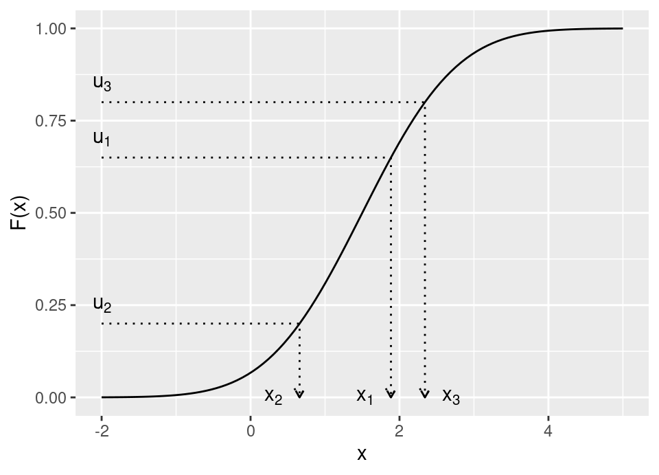
Therefore, the following is a valid cdf and our inverse transform sampling must accommodate the jump discontinuity and region of zero gradient:
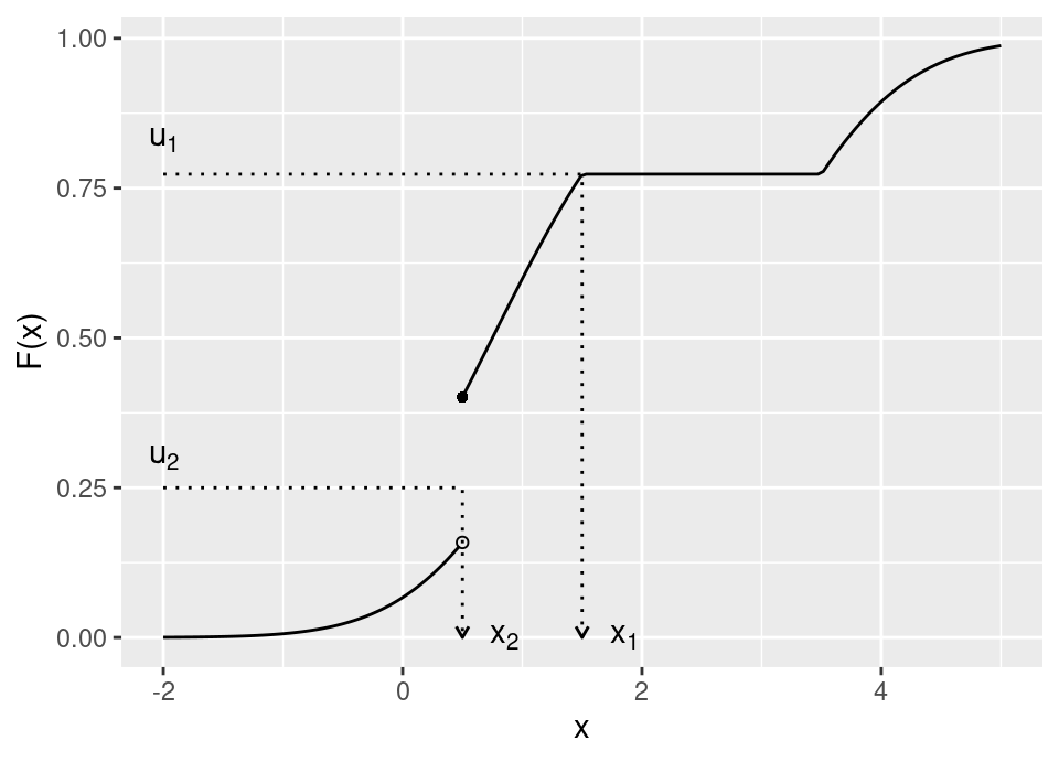
The above cdf has a discrete mass of probability at \(x=0.5\), and a region of zero probability in \(x \in [1.5,3.5]\). The arrows on the graph show how we propose to deal with such situations. More formally,
Definition 5.2 (Generalised inverse cdf) Let \(F(\cdot)\) be a cdf. Then the generalised inverse cdf is given by, \[F^{-1}(u) := \inf \{ x : F(x) \ge u \}, \ \forall\ u\in[0,1]\]
We can now proceed to prove the validity of inverse transform sampling.
Theorem 5.1 Let \(F(\cdot)\) be a cumulative distribution function, having generalised inverse \(F^{-1}(\cdot)\).
If \(U \sim \textrm{Unif}(0,1)\) and \(X = F^{-1}(U)\), then \(X \sim F\).
Proof. We know (Prob I) that the cumulative distribution function completely determines the distribution of \(X\), so if we can compute the cdf, \(\mathbb{P}(X \le x)\), of the random value generated by this algorithm and show that this equals \(F(\cdot)\), then we know we have generated a sample with the correct distribution.
First, by the definition of the generalised inverse cdf, we have that \[F^{-1}(u) \le x \iff u \le F(x)\]
Therefore, we can derive the cdf of \(X\) as, \[\begin{align*} \mathbb{P}(\, X \le x \,) &= \mathbb{P}(\, F^{-1}(U) \le x \,) \\ &= \mathbb{P}(\, U \le F(x) \,) \\ &= F(x) \end{align*}\] Therefore, the cdf of \(X\) is \(F(\cdot)\) as required.
Example 5.1 (Inverse transform sampling a Weibull random variable) In order to use inverse transform sampling for a Weibull distribution with shape \(k\) and scale \(\sigma\), \(X \sim \mathrm{Weibull}(k, \sigma)\), note that: \[\begin{align*} f(x) &= \frac{k}{\sigma} \left( \frac{x}{\sigma} \right)^{k-1} e^{-\left( \frac{x}{\sigma} \right)^k}, \quad x \in [0, \infty), \sigma>0, k>0 \\ F(x) &= 1 - \exp\left\{-\left( \frac{x}{\sigma} \right)^k\right\} \end{align*}\] To find \(F^{-1}(u)\), set \(1 - \exp\left\{-\left( \frac{x}{\sigma} \right)^k\right\} = u\) and solve for \(x\): \[\implies x = F^{-1}(u) = \sigma \left( -\log(1-u) \right)^{1/k}\] In order to generate samples from the Weibull we therefore take values, \(u\), from a Uniform random number stream and transform them using this generalised inverse cdf.
# Sample 10,000 uniforms
u <- runif(10000)

# Compute generalised inverse of Weibull on those uniform draws
# We take parameters k = 1.5, sigma = 1.5
k <- 1.5
sigma <- 1.5
x <- sigma*(-log(1-u))^(1/k)

# Let's compare the histogram of these samples with the exact
# density of a Weibull (in red)
library("ggplot2")

ggplot(data.frame(x = x)) +
  xlim(0, 4) +
  geom_histogram(aes(x = x, y = after_stat(density))) +
  geom_function(fun = function(x) { dweibull(x, shape = k, scale = sigma) }, colour = "red")
Example 5.2 (Inverse transform sampling a Geometric random variable) The Geometric distribution is a countably infinitely supported discrete distribution, \[\begin{align*} f(x) &= \theta (1-\theta)^x, \quad x \in \{0, 1, 2, 3, ...\}, \theta \in [0,1] \\ F(x) &= 1 - (1-\theta)^{x+1} \end{align*}\]
We need to be a little careful, because the cdf is actually a step function, so might more accurately be written: \[F(x) = 1 - (1-\theta)^{\lfloor x+1 \rfloor}\]
The following plot shows in black this cdf, and in pale green the same function without the floor operation to round down:
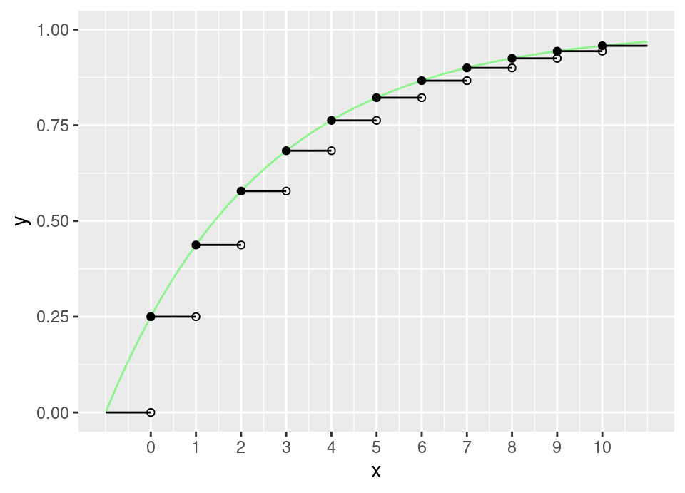
Now to perform inverse transform sampling, we must find \(F^{-1}(u)\). This is more easily done for the continuous version, then taking the appropriate ceiling or floor operation at the end. Set \(1 - (1-\theta)^{x+1} = u\) and solve for \(x\): \[\begin{align*} \implies (1-\theta)^{x+1} &= 1 - u \\ \implies (x+1) \log (1-\theta) &= \log (1-u) \\ \implies x &= \frac{\log (1-u)}{\log (1-\theta)} - 1 \\ \end{align*}\] We can see from the graph that we must take the ceiling operation to correctly agree with the generalised inverse cdf. However, we can slightly simplify further by noting:
- If \(U \sim \text{Unif}(0,1)\), then \(1-U \sim \text{Unif}(0,1)\) also. Therefore, we can just take \(\log u\) in the numerator.
- \(\lceil y - 1 \rceil = \lfloor y \rfloor\) at non-integer values (and sampling an exact integer is a probability zero event).
Thus, \[x = \left\lfloor \frac{\log u}{\log (1-\theta)} \right\rfloor\]
# Sample 10,000 uniforms
u <- runif(10000)

# Compute generalised inverse of Geometric on those uniform draws
# We take parameter theta = 0.2
theta <- 0.2
x <- floor(log(u)/log(1-theta))

# Let's compare the histogram of these samples with the exact
# mass function of a Geometric (in red)
library("ggplot2")

# Note we need to be very careful about how ggplot makes the histogram
# for a problem like this, and specify the bin construction exactly
ggplot(data.frame(x = x)) +
  xlim(0, 20) +
  geom_histogram(aes(x = x, y = after_stat(density)), binwidth = 1, boundary = 0, closed = "left") +
  geom_step(aes(x = x, y = y),
            data.frame(x = 0:20, y = dgeom(0:20, theta)),
            colour = "red")
Inverse transform sampling is a handy method for many standard univariate probability distributions and indeed many standard probability distributions can be sampled (like those in R) using this approach. We will want more general methods, but often those will rely on sampling from a standard distribution, which means inverse transform sampling is often “hidden” within more complex algorithms. In particular, it is more often the case that we know the pdf and not the cdf (and if we could integrate the pdf to get the cdf, then it might well be possible to avoid using simulation in many settings!)
5.2 Rejection sampling
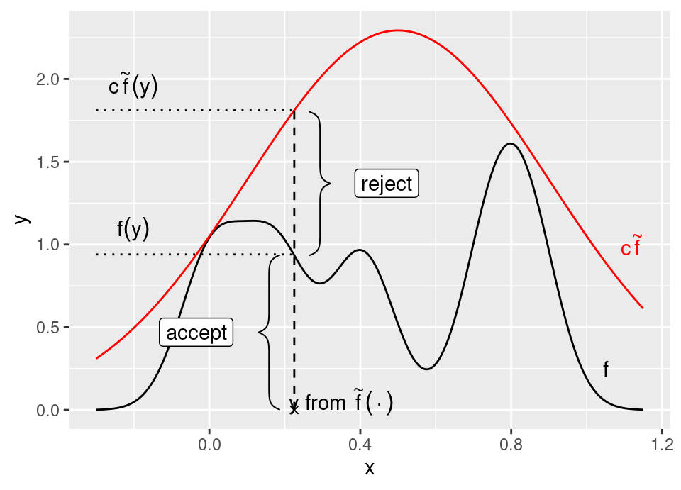
The inverse transform sampling method is really limited to 1-dimensional distributions, though various extensions to higher dimensions have been proposed. Our first higher dimensional method is an elegant algorithm, which actually still crops up in more advanced guises at the cutting edge of modern Monte Carlo research! Rejection sampling just requires the probability density function, \(f(\cdot)\), and not the cdf. If we are doing, say, Monte Carlo integration then this matters a lot, because if we could integrate \(f(\cdot)\) to get the cdf then we might not have needed Monte Carlo at all!
The goal is to find another distribution, say \(\tilde{f}(\cdot)\), which is easier to sample from (perhaps using inverse transform sampling!) and where we can construct a bound on the density function: \[f(x) \le c \tilde{f}(x) \quad\forall\,x \in \mathbb{R}^d\] where \(c < \infty\). We call \(\tilde{f}(\cdot)\) the proposal density, since samples will be drawn from this and then exactly the correct proportion of them retained in order to end up with a stream of samples from \(f(\cdot)\). We call \(f(\cdot)\) the target density, since we ‘aim’ our accepted samples to come from it.
Definition 5.3 (Rejection sampling) Given a (possibly un-normalised) probability density function \(f(\cdot)\), and a (possibly un-normalised) proposal density \(\tilde{f}(\cdot)\), satisfying \(f(x) \le c \tilde{f}(x) \ \forall\,x \in \mathbb{R}^d\) for some \(c < \infty\), a rejection sample is generated by:
- \(a \gets \mathrm{FALSE}\)
- While \(a = \mathrm{FALSE}\), then
- \(u \sim \mathrm{Unif}(0,1)\)
- \(x \sim \tilde{f}(\cdot)\)
- If \(u \le \frac{f(x)}{c \tilde{f}(x)}\) then set \(a \gets \mathrm{TRUE}\)
- Once the while loop is exited, return the sample \(x\).
The value \(x\) will be a realisation of a simulation from \(f(\cdot)\).
Important note: \(f\) and \(\tilde{f}\) need not be normalised probability densities (ie they don’t have to integrate to 1, though obviously they must be non-negative and with finite integral).
There is a nice geometric interpretation of rejection sampling, which can be seen with a simple rearrangement of the acceptance condition: \[\begin{align*} u &\le \frac{f(x)}{c \tilde{f}(x)} \\ \iff u \left( c \tilde{f}(x) \right) &\le f(x) \\ \iff \tilde{u} &\le f(x) \end{align*}\] where \(\tilde{u}\) is a uniform draw on the interval \(\left[ 0,c \tilde{f}(x) \right]\). In other words, we propose a location \(x\) according to \(\tilde{f}(\cdot)\), then draw a Uniform random point vertically between zero and the scaled proposal, accepting it if that draw falls below the target distribution \(f(\cdot)\).
For now, we will proceed based on the assumption that \(f(\cdot)\) and \(\tilde{f}(\cdot)\) are normalised densities (it is a simple change to the following to generalise).
The efficiency of the algorithm hinges entirely on the value of \(c\), so \(\tilde{f}(\cdot)\) should be chosen to make it as small as possible.
Lemma 5.1 When proposal and target are normalised pdfs, the expected number of iterations of the rejection sampling algorithm required before a proposal is accepted is \(c\).
Proof. Let \(A\) be the random variable indicating acceptance of a proposed sample \(X\). Then, the acceptance probability is (abusing notation to aid intuition): \[\begin{align} \mathbb{P}(A = 1) &= \int_\Omega \underbrace{\mathbb{P}(A = 1 \given X = x)}_{\text{Prob A is TRUE for proposed point.}}\ \underbrace{\mathbb{P}(X = x)}_{\text{Proposal density $\tilde{f}$.}} \,dx \\ &= \int_\Omega \underbrace{\mathbb{P}\left(U \le \frac{f(x)}{c \tilde{f}(x)}\right)}_{\text{Uniform cdf, $\mathbb{P}(U \le u) = F(u) = u$.}}\ \tilde{f}(x) \,dx \\ &= \int_\Omega \frac{f(x)}{c \tilde{f}(x)}\ \tilde{f}(x) \,dx \\ &= \frac{1}{c} \int_\Omega f(x) \,dx \\ &= \frac{1}{c} \end{align}\] where \(\Omega\) is the support of \(\tilde{f}(\cdot)\), \(\tilde{f}(x)>0, \ \forall\ x\in \Omega\). The final line follows because the integral of a density over the whole space is 1.
Hence, the number of iterations of the while loop which must be performed in rejection sampling to return a single sample from \(f(\cdot)\) is Geometrically distributed with parameter \(\frac{1}{c}\). Therefore, the expected number of random number of iterations of rejection sampling to get an accepted value is \(c\) (since the expectation of a Geometric distribution with parameter \(p\) is \(1/p\)).
So, although there are infinitely many values of \(c\) which may work (since it can be any value large enough), choosing the value which is as small as possible but still provides the bound will give the most efficient rejection sampler. Consequently, not every proposal distribution is equally good for any given problem: we should favour proposal distributions which require a smaller \(c\) to dominate the target.
Important note: You can do rejection sampling (ie compute the required \(c\)) whether or not \(\tilde{f}(\cdot)\) and \(f(\cdot)\) are normalised pdfs … but, \(c\) will only equal the expected number of iterations when both are normalised (otherwise \(c\) also contains some hidden normalising constants).
Theorem 5.2 Let \(f(\cdot)\) and \(\tilde{f}(\cdot)\) be probability density functions satisfying \(f(x) \le c \tilde{f}(x) \ \forall\,x \in \mathbb{R}^d\) for some \(c < \infty\). Then \(X\) generated by algorithm in the definition of rejection sampling has pdf \(f(\cdot)\).
Proof. We note that the samples returned are only those which are accepted, so we condition on this event:
\[\begin{align*} \mathbb{P}(X \in E \given A = 1) &= \frac{\mathbb{P}(A = 1 \given X \in E)\ \mathbb{P}(X \in E)}{\mathbb{P}(A = 1)} && \forall\ E \in \mathcal{B} \\ &= \frac{\int_E \frac{f(x)}{c \tilde{f}(x)} \ \tilde{f}(x) \,dx}{\frac{1}{c}} \\ &= \int_E f(x) \,dx \end{align*}\] The last line is the probability of event \(E\) under the distribution with density \(f(\cdot)\), as required.
Important note: not every distribution can act as a proposal for every target! Sometimes an appropriate \(c\) simply does not exist. Most commonly, this failure happens due to behaviour in one or both tails (ie as \(x \to \pm \infty\)).
Example 5.3 (Failure of rejection sampling) Imagine that we cannot inverse transform sample a Pareto random variable (we can, in fact). The pdf of the Pareto with scale parameter \(\eta > 0\) and shape parameter \(\alpha > 0\) is:
\[f(x) = \alpha \eta^\alpha x^{-\alpha-1} \quad \forall\,x\in[\eta,\infty)\]
Assume \(\eta = 1\), then we may think to use simulations from an Exponential distribution to rejection sample from the Pareto. However,
\[\begin{align*} f(x) &\le c \tilde{f}(x) \quad\forall\ x \in \mathbb{[0,\infty)} \\ \implies \alpha x^{-\alpha-1} &\le c \lambda e^{-\lambda x} \\ \implies \frac{\alpha}{\lambda} x^{-\alpha-1} e^{\lambda x} &\le c \end{align*}\]
Here, as \(x \to \infty\), the exponential term will grow faster than the reciprocal polynomial term in \(x\), so that in the right tail \(c \to \infty\). In other words, there is no choice \(c < \infty\) which ensures an Exponential pdf bounds a Pareto pdf and hence we cannot perform rejection sampling from a Pareto with this proposal (we must find a proposal with so-called “heavier tails” so that it can dominate on the whole non-negative real line).
Example 5.4 (Rejection sampling Normal with Cauchy) The standard Normal distribution has a closed form pdf:
\[f(x) = \frac{1}{\sqrt{2 \pi}} e^{-\frac{x^2}{2}}\]
However, it does not have a closed form expression for the cdf, so standard inversion sampling as described above would not seem to be possible. Therefore we might choose to try rejection sampling.
Consider the Cauchy distribution with scale parameter \(\gamma\) and location parameter \(\eta\), which has pdf:
\[\tilde{f}(x) = \frac{1}{\pi \gamma\left( 1+ \left(\frac{x - \eta}{\gamma}\right)^2 \right)}, \quad x \in \mathbb{R}\]
The standard Cauchy distribution is defined to be when \(\gamma = 1, \eta = 0\), so that:
\[\begin{align*} \tilde{f}(x) &= \pi^{-1} (1+x^2)^{-1} \\ \tilde{F}(x) &= \int_{-\infty}^x \pi^{-1} (1+z^2)^{-1} \,dz \\ &= \Big. \pi^{-1} \arctan z \Big|_{-\infty}^x \\ &= \pi^{-1} \arctan x + \frac{1}{2} \end{align*}\]
Therefore, we can use inverse transform sampling to generate Cauchy distributed random simulations by sampling \(U \sim \text{Unif}(0,1)\) and computing \(X = \tan\left(\pi(U-0.5)\right)\).
Can we use these standard Cauchy simulations in a rejection sampler to generate standard Normal simulations? To be able to do so, we would require a \(c<\infty\) such that:
\[\begin{align*} f(x) &\le c \tilde{f}(x) \quad\forall\ x \in \mathbb{R} \\ \implies \frac{1}{\sqrt{2 \pi}} e^{-\frac{x^2}{2}} &\le c \left( \pi^{-1} (1+x^2)^{-1} \right) \\ \implies \pi (1+x^2) (2 \pi)^{-1/2} \exp\left(-\frac{x^2}{2}\right) &\le c \end{align*}\]
In other words, we require:
\[c = \sup_{x \in \mathbb{R}} \sqrt{\frac{\pi}{2}} (1+x^2) \exp\left(-\frac{x^2}{2}\right)\]
Firstly, note that as \(x \to \pm \infty\), the exponential will decay faster than the quadratic grows, so the expression tends to zero in the tails.
Thus we can look at the behaviour in the body of the distribution. The first and second derivatives of the right hand can be found using the product rule to get:
\[\begin{align*} \frac{d}{dx} &= - \sqrt{\frac{\pi}{2}} \exp\left(-\frac{x^2}{2}\right) x (x^2 - 1) \\ \frac{d^2}{dx^2} &= \sqrt{\frac{\pi}{2}} \exp\left(-\frac{x^2}{2}\right) \left( x^4 - 4 x^2 + 1\right) \end{align*}\]
By inspection, \(d/dx = 0 \iff x \in \{ -1, 0, 1 \}\). Using the second derivative, we can see that \(d^2/dx^2 < 0\) for \(x \in \{ -1, 1 \}\) and \(d^2/dx^2 > 0\) for \(x = 0\). Hence, the supremum is attained at \(x = \pm 1\) and clearly will have the same value for both \(x\).
Therefore, \(c \approx 1.521\) (NB: always round up the least significant digit being retained, because \(c\) must satisfy the rejection sampling inequality).
Hence, we can use simulations from a standard Cauchy distribution to generate simulations from a standard Normal distribution using rejection sampling. The efficiency of the rejection sampler is such that the acceptance probability for each iteration is about \(0.6577\).
For example, to generate 10,000 simulations we would therefore expect on average to need to do 15,210 proposals since on average 5,210 would be rejected.
library("ggplot2")

# Define the pdfs (these are built into R, but we want to show details)
normal_pdf <- function(x) {
  1/sqrt(2*pi)*exp(-x^2/2)
}
cauchy_pdf <- function(x) {
  1/(pi*(1+x^2))
}

# Check that C*(Cauchy pdf) does indeed dominate the Normal
C <- sqrt(pi/2)*(1+1)*exp(-1/2)

ggplot() +
  xlim(-4, 4) +
  geom_function(fun = cauchy_pdf, colour = "green") +
  geom_function(fun = normal_pdf, colour = "red") +
  geom_function(fun = function(x) { C*cauchy_pdf(x) }, colour = "blue") +
  labs(title = "Check if C*Cauchy (blue) dominates Normal (red). 1*Cauchy in green")

# Looks good, so proceed to rejection sampling
x <- rep(0, 10000) # Store Normal draws
x2 <- c() # Store Cauchy draws
for(i in 1:10000) {
  accept <- FALSE
  while(!accept) {
    # Inverse sample to get Cauchy proposal, x_prop
    u1 <- runif(1)
    x_prop <- tan(pi*(u1-0.5))

    # Save the Cauchy draws to check their distribution later
    x2 <- c(x2, x_prop)

    # Test for acceptance/rejection of x_prop
    u2 <- runif(1)
    if(u2 < normal_pdf(x_prop)/(C*cauchy_pdf(x_prop))) {
      accept <- TRUE
    }
  }
  x[i] <- x_prop
}

# Let's compare the histogram of:
#   - inverse samples with exact standard Cauchy
#   - rejection samples with exact standard Normal
library("ggplot2")

ggplot(data.frame(x = x2)) +
  xlim(-8, 8) +
  geom_histogram(aes(x = x, y = after_stat(density))) +
  geom_function(fun = cauchy_pdf, colour = "red") +
  labs(title = "Check of inverse sampled Cauchy draws")

ggplot(data.frame(x = x)) +
  geom_histogram(aes(x = x, y = after_stat(density))) +
  geom_function(fun = normal_pdf, colour = "red") +
  labs(title = "Check of rejection sampled Normal draws")
5.3 Importance sampling
The final core standard Monte Carlo method we cover also starts from the perspective of having a proposal density \(\tilde{f}(\cdot)\), though we no longer require it to be able to bound \(f(\cdot)\). Importance sampling then dispenses with the notion of directly generating iid samples from \(f(\cdot)\) and focuses on their use: as we saw at the end of the last Chapter, all quantities of interest boil down to computation of expectations using those samples.
\[\mu := \mathbb{E}[g(X)] = \int g(x) f_X(x)\,dx \approx \frac{1}{n} \sum_{i=1}^n g(X_i) =: \hat{\mu} \ \text{ where }\ X_i \sim f_X(\cdot)\]
Inverse sampling and rejection sampling focused on directly generating the required \(X_i \sim f_X(\cdot)\). However, importance sampling instead takes samples from the proposal \(\tilde{f}(\cdot)\) and always keeps them, simply weighting to adjust the contribution of each sample to the expectation estimator so that they actually equal the expectation under \(f(\cdot)\). As such, an importance sample consists not just of a random draw, but also of a weight: \((x, w)\).
Note that importance sampling requires real care in application. Inverse sampling “just works” if we can do the algebra, and rejection sampling “just works” if we have correctly found the bound (though may be slow if the acceptance probability is too small), but importance sampling can completely fail (and silently) if we are not careful! The trade-off is that when it is applied correctly, importance sampling can be dramatically more efficient than rejection sampling, so much so that it forms the backbone of many much more advanced methods which we won’t have time to cover in this course.
We will examine two variants of importance sampling: a standard method for correctly normalised target (\(f\)) and proposal (\(\tilde{f}\)) densities, and a self-normalised method for un-normalised target and proposal densities.
5.3.1 Normalised Importance Sampling
Definition 5.4 (Importance sampling) Given a correctly normalised probability density function \(f(\cdot)\), and a correctly normalised proposal density \(\tilde{f}(\cdot)\), we produce \(n\) importance samples by the following steps:
For \(i \in \{1, \dots, n\}\)
- Generate \(x_i \sim \tilde{f}(\cdot)\)
- Compute \(w_i = \frac{f(x_i)}{\tilde{f}(x_i)}\)
Then, \(\{ (x_i, w_i) \}_{i=1}^n\) are importance samples from \(f(\cdot)\) and the importance sampling estimate of \(\mu = \mathbb{E}[g(X)]\) is given by: \[\hat{\mu} = \frac{1}{n} \sum_{i=1}^n w_i g(x_i)\]
Before we prove that this does indeed give us an estimate of \(\mu\), we need to remind ourselves of the precise definition of expectation. Note, that when we talk about an expectation we really need to specify what it is with respect to. In other words,
\[\mathbb{E}[X h(X)] = \int \big( x h(x) \big) f(x)\,dx\]
is an expectation with respect to \(f(\cdot)\). But, if it so happens that \(\eta(x) := h(x) f(x)\) is a valid probability density function, then we could write:
\[\mathbb{E}_f[X g(X)] = \int \big( x h(x) \big) f(x)\,dx = \int x \big( h(x) f(x) \big)\,dx = \mathbb{E}_\eta[X]\]
In other words, exactly the same value (same integral) can represent an expectation of \(X h(X)\) with respect to \(f(\cdot)\), or an expectation of \(X\) with respect to \(\eta(\cdot)\). To emphasise this, we added the subscript to the expectation operator to show the relevant information.
Theorem 5.3 Let \(\mu := \mathbb{E}_f\left[g(X)\right]\), and let \(\tilde{f}(\cdot)\) be a pdf such that \(\tilde{f}(x) > 0\) whenever \(g(x) f(x) \ne 0\).
Then, for \(\hat{\mu}\) as in Definition 5.4,
\[\mathbb{E}_{\tilde{f}}[\hat{\mu}] = \mu\]
Proof. The Theorem statement is saying that the weighted expectation using simulations from \(\tilde{f}(\cdot)\) will give an unbiased estimate of the true desired expectation with respect to \(f(\cdot)\).
To see that this weighting has the desired effect, consider the expectation which is our objective: \[\begin{align*} \mathbb{E}_f[g(X)] &= \int_\Omega g(x) f(x) \,dx \\ &= \int_\Omega g(x) \frac{\tilde{f}(x)}{\tilde{f}(x)} f(x) \,dx && \text{multiply and divide by $\tilde{f}(x)$} \\ &= \int_{\tilde{\Omega}} \left( g(x) \frac{f(x)}{\tilde{f}(x)} \right) \tilde{f}(x) \,dx \\ &= \mathbb{E}_{\tilde{f}}\left[\frac{g(X) f(X)}{\tilde{f}(X)}\right] \\ &= \mathbb{E}_{\tilde{f}}\left[w(X) g(X) \right] \end{align*}\] where \(w(X) := \frac{f(X)}{\tilde{f}(X)}\) is the weight function, as per Definition 5.4; \(\Omega\) is the support of \(f(\cdot)\); and \(\tilde{\Omega}\) is the support of \(\tilde{f}(\cdot)\).
But, we know from the weak (and strong) law of large numbers that, \[ \hat{\mu} = \frac{1}{n} \sum_{i=1}^n w_i g(x_i) \overset{n\to\infty}{\longrightarrow} \mathbb{E}_{\tilde{f}}\left[w(X) g(X) \right]\] Hence, \[\hat{\mu} \overset{n\to\infty}{\longrightarrow} \mathbb{E}_f[g(X)]\] as required.
Some care is required, because although this estimator is unbiased for the expectation of interest, the variance is no longer going to be the same as the usual Monte Carlo variance where \(x_i \sim f(\cdot)\)!
Theorem 5.4 The variance of the importance sampling estimator is, \[\begin{align*} \mathrm{Var}(\hat\mu) = \frac{\sigma_{\tilde{f}}^2}{n} \ \text{ where } \ \sigma_{\tilde{f}}^2 = \int_{\tilde{\Omega}} \frac{\left( g(x) f(x) - \mu\tilde{f}(x) \right)^2}{\tilde{f}(x)}\,dx, \end{align*}\]
Proof. \[\begin{align*} \mathrm{Var}(\hat\mu) &= \mathrm{Var}\left( \frac{1}{n} \sum_{i=1}^n W_i g(X_i) \right) \\ &= \frac{1}{n^2} \sum_{i=1}^n \mathrm{Var}\left( W_i g(X_i) \right) \\ &= \frac{1}{n^2} n \mathrm{Var}\left( \frac{g(X) f(X)}{\tilde{f}(X)} \right) \\ &= \frac{\sigma_{\tilde{f}}^2}{n} \end{align*}\]
where
\[\begin{align*} \sigma_{\tilde{f}}^2 &= \mathrm{Var}_{\tilde{f}}\left( \frac{g(X) f(X)}{\tilde{f}(X)} \right) \\ &= \mathbb{E}_{\tilde{f}}\left[ \left(\frac{g(X) f(X)}{\tilde{f}(X)}\right)^2 \right] - \mathbb{E}_{\tilde{f}}\left[ \frac{g(X) f(X)}{\tilde{f}(X)} \right]^2 \\ &= \int_{\tilde{\Omega}} \left(\frac{g(x) f(x)}{\tilde{f}(x)}\right)^2 \tilde{f}(x) \,dx - \mu^2 \\ &= \int_{\tilde{\Omega}} \frac{\left(g(x) f(x)\right)^2}{\tilde{f}(x)} \,dx - \mu^2 \int_{\tilde{\Omega}} \frac{\tilde{f}(x)^2}{\tilde{f}(x)} \,dx \\ &= \int_{\tilde{\Omega}} \frac{\left( g(x) f(x) - \mu\tilde{f}(x) \right)^2}{\tilde{f}(x)}\,dx \end{align*}\]
since
\[-\int_{\tilde{\Omega}} \frac{2 g(x) f(x) \mu \tilde{f}(x)}{\tilde{f}(x)}\,dx = -2 \mu \int_{\tilde{\Omega}} g(x) f(x)\,dx = -2\mu^2\]
as required.
We can empirically estimate the required variance from the importance samples using, \[\begin{equation} \hat\sigma_{\tilde{f}}^2 = \frac{1}{n} \sum_{j=1}^n \left( g(x_j) w_j - \hat\mu \right)^2 \label{eq:impsamp-norm-var} \end{equation}\]
As such, just like we saw previously, \(\sigma_{\tilde{f}}^2\) (or its empirical estimate \(\hat\sigma_{\tilde{f}}^2\)) provide a guide to when we have a ‘good’ importance sampling algorithm, since if \(\tilde{f}(\cdot)\) is fixed the only other option to improve the estimate is to increase the simulation size \(n\).
Indeed, it can be shown (a simple application of Cauchy–Schwarz) that the theoretically optimal proposal distribution which minimises the estimator variance is: \[ \tilde{f}_{\mathrm{opt}}(x) = \frac{ |g(x)| f(x) }{ \int_\Omega |g(x)| f(x)\,dx } \] In particular, note that this implies that importance sampling can achieve super-efficiency whereby it results in lower variance even than sampling directly from \(f(\cdot)\) when \(g(x) \ne x\). In particular, if \(g(x) \ge 0 \ \forall x\) then this proposal results in a zero-variance estimator! Of course, in practice we can never sample from and evaluate this optimal proposal, since it is at least as difficult as the original problem we were attempting to solve! However, even though unusable, it provides guidance toward the form of a good proposal for any given importance sampling problem.
The following example highlights that even when we can draw samples from \(f(\cdot)\), for a particular expectation we may still benefit from importance sampling.
Example 5.5 Consider the toy problem of computing \(\mathbb{P}(X > 3.09)\) when \(X\) is a standard Normal random variable. Using R we can accurately find the true answer to this is \(0.001001\) (4 sf). However, since the distribution is not in closed form, let us imagine that we cannot! If we can only compute the Normal density then we might choose to use an inverse sampler to generate Cauchy (see above) or Laplace simulations (Tutorial 5), use these in a rejection sampler to get Normal simulations, then evaluate the above probability using Monte Carlo integration with those Normal simulations.
In other words, simulate many \(x_i \sim \text{N}(0,1)\) via inverse and rejection sampling and then compute \[\mathbb{P}(X > 3.09) = \mathbb{E}\left[\bbone\{ X \in [3.09,\infty)\}\right] = \frac{1}{n} \sum_{j=1}^n \bbone\{ x_j \in [3.09,\infty)\}\] However, this will require very many samples to achieve an accurate estimate of this tail probability. Indeed, we know \(p=0.001001\), so if we wanted 95% confidence in an accuracy to 4 significant figures we would need: \[\begin{align*} 1.96 \sqrt{\frac{p(1-p)}{n}} &= 0.000001 \\ \implies n = 3,841,592,313 \end{align*}\]
In contrast, still only using simulations from a Normal distribution, we may elect to use importance sampling with a proposal \(\tilde{f}(\cdot)\) which is \(\text{N}(m, 1)\) for some choice \(m\) (Note: we just add \(m\) to standard Normal simulations to get this). To select \(m\), we could perform a small grid search over possible proposals, computing \(\hat\sigma_{\tilde{f}}^2\) each time, to find a good choice, as in the following code.
# Define the pdfs (these are built into R, but we want to show details)
# This time we need the mean of the Normal due to the Importance Sampling proposal
normal_pdf <- function(x, mu = 0) {
  1/sqrt(2*pi)*exp(-(x-mu)^2/2)
}
cauchy_pdf <- function(x) {
  1/(pi*(1+x^2))
}

# C as found in earlier example
C <- sqrt(pi/2)*(1+1)*exp(-1/2)

# Rejection sampling
x <- rep(0, 10000) # Store Normal draws
for(i in 1:length(x)) {
  accept <- FALSE
  while(!accept) {
    # Inverse sample to get Cauchy proposal, x_prop
    u1 <- runif(1)
    x_prop <- tan(pi*(u1-0.5))

    # Test for acceptance/rejection of x_prop
    u2 <- runif(1)
    if(u2 < normal_pdf(x_prop)/(C*cauchy_pdf(x_prop))) {
      accept <- TRUE
    }
  }
  x[i] <- x_prop
}

# Compute the importance sampling variance for some choices of m
m <- seq(1.5, 4.5, length.out = 25)
is_var <- rep(0, length(m))
for(i in 1:length(m)) {
  x_is_prop <- x + m[i]
  w <- normal_pdf(x_is_prop)/normal_pdf(x_is_prop, mu = m[i])
  mu_hat <- mean(I(x_is_prop>3.09)*w)
  is_var[i] <- mean((w*I(x_is_prop>3.09)-mu_hat)^2)
}

lowest <- m[which.min(is_var)]

library("ggplot2")

ggplot(data.frame(m = m, is_var = is_var)) +
  geom_point(aes(x = m, y = is_var)) +
  xlab("m") +
  ylab("Variance of Imp Samps") +
  geom_vline(xintercept = lowest, colour = "red") +
  labs(title = paste0("Lowest IS variance when proposal m = ", lowest))
You should find a value near \(m=3.25\) is found (might differ a bit due to random variation).
We can then use this proposal to do a larger final importance sampling simulation run of, say, \(n=100,000\). To compare, we use the same random number stream to create a naive Monte Carlo, and you will see a substantial difference in accuracy!
# Define the pdfs (these are built into R, but we want to show details)
# This time we need the mean of the Normal due to the Importance Sampling proposal
normal_pdf <- function(x, mu = 0) {
  1/sqrt(2*pi)*exp(-(x-mu)^2/2)
}
cauchy_pdf <- function(x) {
  1/(pi*(1+x^2))
}

# C as found in earlier example
C <- sqrt(pi/2)*(1+1)*exp(-1/2)

# Rejection sampling
x <- rep(0, 100000) # Store Normal draws
for(i in 1:length(x)) {
  accept <- FALSE
  while(!accept) {
    # Inverse sample to get Cauchy proposal, x_prop
    u1 <- runif(1)
    x_prop <- tan(pi*(u1-0.5))

    # Test for acceptance/rejection of x_prop
    u2 <- runif(1)
    if(u2 < normal_pdf(x_prop)/(C*cauchy_pdf(x_prop))) {
      accept <- TRUE
    }
  }
  x[i] <- x_prop
}

cat("Based on an identical number of simulations, we have:")

# Naive estimator
mu_hat_naive <- mean(I(x>3.09))
var_naive <- mu_hat_naive*(1-mu_hat_naive)

cat("Naive estimate is:\n  mu.hat =",
    mu_hat_naive,
    "with 95% confidence interval width",
    1.96*sqrt(var_naive/length(x)))

# Importance sampling estimator
m <- 3.25 # You may get slightly different answer from previous code box
x_is_prop <- x + m
w <- normal_pdf(x_is_prop)/normal_pdf(x_is_prop, mu = m)
mu_hat_is <- mean(I(x_is_prop>3.09)*w)
is_var <- mean((w*I(x_is_prop>3.09)-mu_hat_is)^2)

cat("Importance sampling estimate is:\n  mu.hat =",
    mu_hat_is,
    "with 95% confidence interval width",
    1.96*sqrt(is_var/length(x)))

cat("Confidence interval of naive estimator is about",
    round((1.96*sqrt(var_naive/length(x)))/(1.96*sqrt(is_var/length(x)))),
    "times larger than for the importance sampling estimator.")
One may reasonably object that we have ignored the 25 pilot runs of \(n=10,000\) importance samples used to select \(m=3.25\), so that the total computational effort expended on importance sampling was at least \(3.5\times\) that of standard Monte Carlo. However, even accounting for the pilot computational effort to select a proposal distribution, there is substantial benefit to using importance sampling as seen by the fact that the naive method has about a \(17\times\) larger confidence interval.
5.3.2 Self-normalised Importance Sampling
We can use un-normalised proposals too via the following self-normalising algorithm:
Definition 5.5 (Self-normalised importance sampling) Given a (possibly un-normalised) probability density function \(f(\cdot)\), and a (possibly un-normalised) proposal density \(\tilde{f}(\cdot)\), self-normalised importance sampling produces importance samples \(\{ (x_i, w_i) \}_{i=1}^n\) as described in Definition 5.4, but the importance sampling estimate of \(\mu = \mathbb{E}[g(X)]\) is modified to: \[\hat{\mu} = \frac{\sum_{i=1}^n w_i g(x_i)}{\sum_{i=1}^n w_i}\]
However, it is important to note that this estimator is no longer unbiased, though asymptotically it is. Additionally, the variance of this estimator is more complicated having only approximate form. An approximate estimate can be computed using, \[\begin{align*} \mathrm{Var}(\hat{\mu}) \approx \frac{\hat{\sigma}_{\tilde{f}}^2}{n} \ \text{ where } \ &\hat{\sigma}_{\tilde{f}}^2 = \sum_{j=1}^n w_j'^{2} \left( g(x_j) - \hat\mu \right)^2 \\ \text{ and } \ &w_j' = \frac{w_j}{\sum_{i=1}^n w_i} \end{align*}\]
Finally, the theoretically optimal (but unusable) proposal in the self-normalised weight case is, \[\tilde{f}(x)_{\mathrm{opt}} \propto |g(x) - \mu| f(x)\]
5.3.3 Diagnostics
Additional care is required in the application of importance sampling when compared to using iid samples from the distribution of interest. In particular, because importance sampling uses a weighted collection of samples, it is not uncommon to be in a situation where a small number of samples with large weight dominate the estimate, so that simply having many importance samples does not equate to good estimation overall.
A common diagnostic for potential weight imbalance is derived by equating the variance of a weighted importance sampling approach to the naive iid Monte Carlo variance for an average computed using a fixed but unknown sample size \(n_e\). With simple algebraic rearrangement one may then solve for \(n_e\), the so-called effective sample size. This informally corresponds to the size of a naive iid Monte Carlo sample one would expect to need to attain the same variance achieved via this importance sample, so that a low value indicates poor weight behaviour (since that corresponds to few iid samples). \[\begin{align*} \mathrm{Var}\left( \frac{\sum_{i=1}^n g(x_i) w_i}{\sum_{i=1}^n w_i} \right) &= \frac{\sigma^2}{n_e} \\ \implies \frac{\mathrm{Var}\left( \sum_{i=1}^n g(x_i) w_i \right)}{\left(\sum_{i=1}^n w_i\right)^2} &= \frac{\sigma^2}{n_e} \\ \implies \frac{\sigma^2 \sum_{i=1}^n w_i^2}{\left(\sum_{i=1}^n w_i\right)^2} &= \frac{\sigma^2}{n_e} \\ \implies n_e &= \frac{n \bar{w}^2}{\overline{w^2}} \end{align*}\] where \[\bar{w}^2 = \left( \frac{1}{n} \sum_{j=1}^n w_j \right)^2 \quad\text{and}\quad \overline{w^2} = \frac{1}{n} \sum_{j=1}^n w_j ^2\]
The reason to use such a diagnostic and not simply rely on the empirical variance estimates above is that they are themselves based on the sampling procedure and therefore may be poor estimates too.
Finally, it is critical to note that although small \(n_e\) does diagnose a problem with importance sampling, it is not necessarily true that large \(n_e\) means everything is ok: it is, for example, entirely possible that the sampler has missed whole regions of high probability.
Example 5.6 We can empirically explore one of the issues that typically causes problems. One of the key reasons importance sampling may fail is if your proposal distribution has much less probability in the tails of the distribution than your target.
For example, we know the \(t\)-distribution is much heavier in the tails than the Normal distribution:
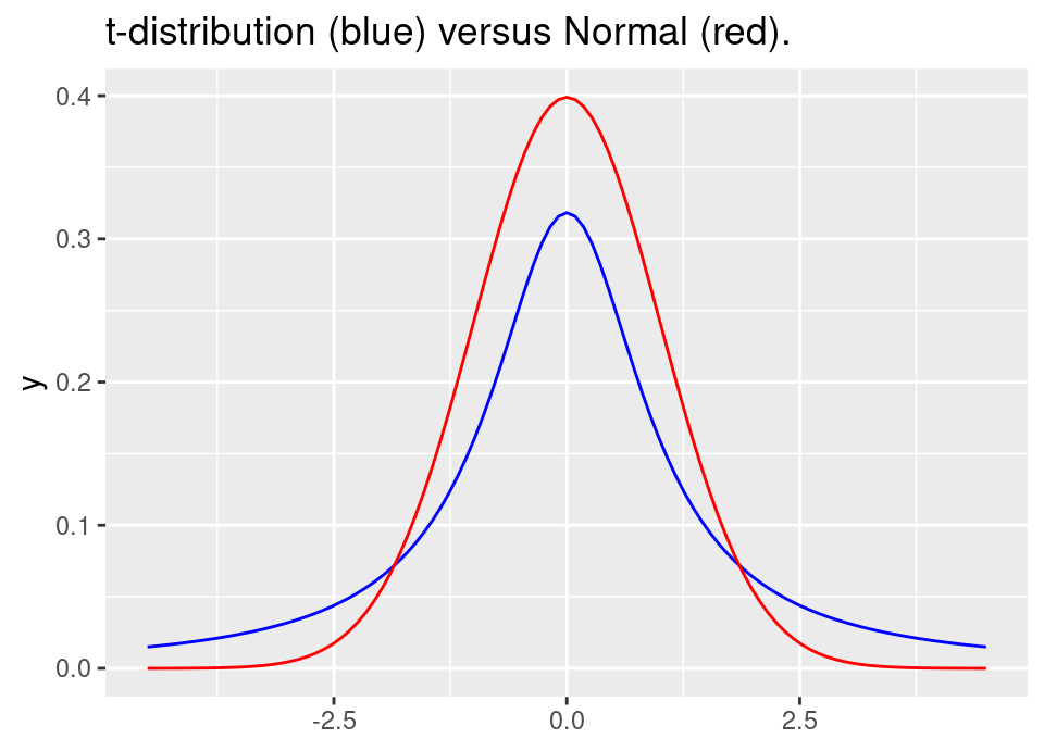
This means that the \(t\)-distribution will be ok as a proposal for the Normal, but not vice-versa. The following code uses the effective sample size to demonstrate this:
# t proposal, Normal target
x <- rt(10000, 1)
w <- dnorm(x)/dt(x, 1)
n_e <- (length(x) * mean(w)^2)/mean(w^2)
cat("ESS for 1000 simulations with a t proposal for a Normal target:", n_e)

# Normal proposal, t target
x <- rnorm(10000)
w <- dt(x, 1)/dnorm(x)
n_e <- (length(x) * mean(w)^2)/mean(w^2)
cat("ESS for 1000 simulations with a Normal proposal for a t target:", n_e)
# NB may need to run multiple times ... note how much the second ESS varies!
Make sure you run the above multiple times. You should find that using 10000 simulations, the ESS for a \(t\) proposal for a Normal target is pretty stable around 7500. However, the ESS for a Normal proposal for a \(t\) target will vary wildly, sometimes being up around 5000 and sometimes dropping into just hundreds. This is because the Normal proposal is too narrow to reliably estimate the behaviour of the \(t\)-distribution in the tails, whilst the \(t\)-distribution provides good coverage of the regions of high probability in a Normal.