Lab 5: Data Visualisation (base)
🧑💻 Make sure to finish earlier Labs before continuing with this lab! It might be tempting to skip some stuff if you’re behind, but you may just end up progressively more lost … we will happily answer questions from any lab each week 😃
5.5 Movies 🎞️ data
The Internet Movie Database (IMDB, imdb.com) is a fantastic resource for film buffs.
A snapshot of data on a large number of films was “web scraped” and and has been made available in the R package ggplot2movies.
You might have seen a similar data set in Stats II recently (if you take it), but it’s too good not to look at again here in DSSC slightly differently!
In real life data science such as you might encounter in your careers after University, there are all sorts of odd things that can get thrown up at you, so part of this course is getting used to spotting and handling these things, as well as developing a healthy inquisitiveness to dig deep into data you work with.
Exercise 5.43 First, we need to get hold of and load data:
- Install the package
ggplot2moviesfrom CRAN; - Load the dataset called
movieswhich is in that package;
Click for solution
## SOLUTION i.

install.packages("ggplot2movies")
## SOLUTION ii.
data("movies", package = "ggplot2movies")Exercise 5.44 Load the help file and read about the variables in the data. How many films are in this data set according to the documentation? Check the dataset, does this agree?
Click for solution
## SOLUTION

# Look in the help file
?ggplot2movies::movies
The help file reports there are 28,819 films in the dataset. Since this is a data frame, we know that observations are in rows, variables are in columns, so to check the actual data that was loaded we just need to see how many rows there are:
nrow(movies)[1] 58788Exercise 5.45 What is the largest budget in the data set?
Click for solution
## SOLUTION

# We can just run the max directly on the budget variable.
max(movies$budget)
[1] NA# Ah! We have run into trouble because some of the budgets must be missing (NA)
# Missing data happens in real world data outside the classroom and is a real
# pain, but fortunately saw with the mean function back in the first lecture we
# could use na.omit on the vector before passing to the function, or use the
# na.rm argument (if you look at the documentation ?max you'll see max has the
# same option)
max(movies$budget, na.rm = TRUE)[1] 200000000max(na.omit(movies$budget))[1] 200000000Exercise 5.46 First subset all the data to eliminate any movies with no budget by running the following code:
movies.withbudget <- movies[!is.na(movies$budget),]Then identify the name of the movie with the highest budget by querying the movies.withbudget data frame.
Click for solution
You might wonder why the question tells us to subset the data first.
Can’t we just do a query for the film with budget equal to $200 millon?
Unfortunately, the usual method of subsetting in R doesn’t play well with missing values, because it will create a whole missing row when you try to match 200000000 against an NA.
For example, try running the following (it is huge so the output is not embedded in these solutions)
## NOT THE SOLUTION(!)

movies[movies$budget==200000000,]
To understand what is happening, as regularly advised in lectures, break it down and look at what happens for just this:
movies$budget==200000000We’ll learn methods that handle this much more gracefully in the coming weeks!
For now, let’s follow the advice of the question and get rid of the rows with an NA budget before trying to identify the big budget movie.
## SOLUTION

movies.withbudget[movies.withbudget$budget==200000000,]
title year length budget rating votes r1 r2 r3 r4 r5 r6
48518 Spider-Man 2 2004 127 200000000 7.9 40256 4.5 4.5 4.5 4.5 4.5 4.5
52348 Titanic 1997 194 200000000 6.9 90195 14.5 4.5 4.5 4.5 4.5 4.5
r7 r8 r9 r10 mpaa Action Animation Comedy Drama Documentary
48518 14.5 24.5 24.5 24.5 PG-13 1 0 0 0 0
52348 14.5 14.5 14.5 24.5 PG-13 0 0 0 1 0
Romance Short
48518 0 0
52348 1 0The remainder of the questions should be done with the full data, don’t use only the subset of those with a budget! To avoid any accident, you can remove temporary variables once you don’t need them any more. Run the following code to remove the subsetted movies from your environment in R.
rm(movies.withbudget)Exercise 5.47 Create a histogram (see help file hist) of the length (in minutes) of all the films, using the defaults for the plotting function. How do you interpret the plot?
Click for solution
## SOLUTION

hist(movies$length)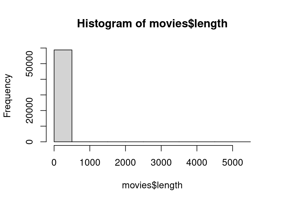
Exercise 5.48 This time, create a boxplot (see help file boxplot) of the length (in minutes) of all the films.
Was your interpretation correct?
What are the names of the unusual films.
Click for solution
## SOLUTION

# Just boxplot would be fine too ... I've used the horizontal option so it looks
# a bit nicer (see the documentation for boxplot!)
boxplot(movies$length, horizontal = TRUE)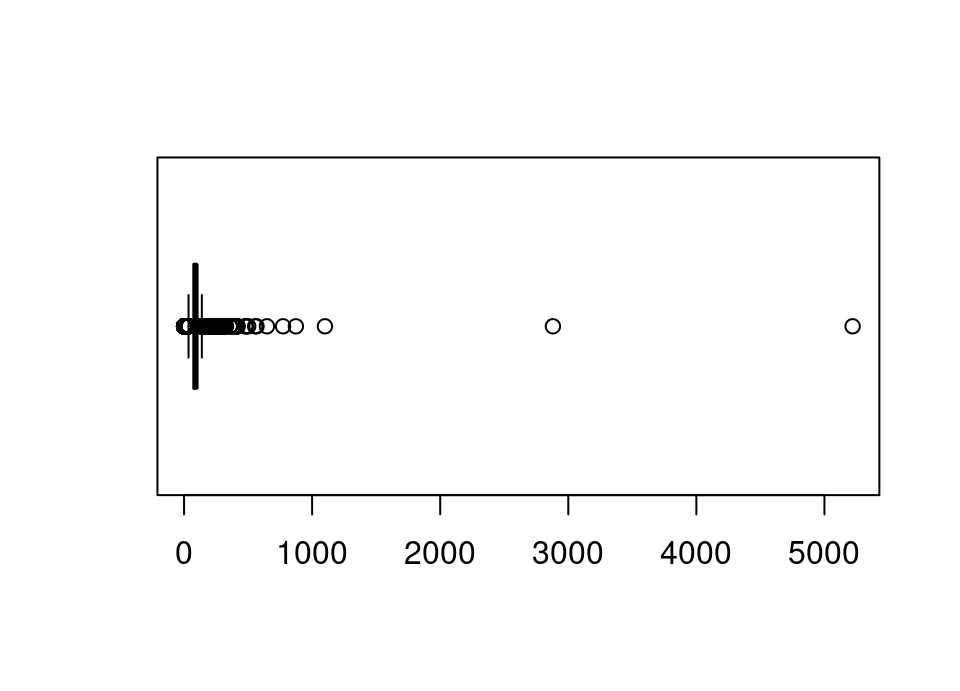
In this instance a boxplot is much better to see what is going on, since any outlying points beyond the right tail are shown as individual points. Amazingly there are 3 films with running times over 1000 minutes (or 16.7 hours!) Let’s look at them:
movies[movies$length > 1000,] title year length budget
11937 Cure for Insomnia, The 1987 5220 NA
18741 Four Stars 1967 1100 NA
30574 Longest Most Meaningless Movie in the World, The 1970 2880 NA
rating votes r1 r2 r3 r4 r5 r6 r7 r8 r9 r10 mpaa Action
11937 3.8 59 44.5 4.5 4.5 4.5 0 0 0.0 4.5 4.5 44.5 0
18741 3.0 12 24.5 0.0 4.5 0.0 0 0 4.5 0.0 0.0 45.5 0
30574 6.4 15 44.5 0.0 0.0 0.0 0 0 0.0 0.0 0.0 64.5 0
Animation Comedy Drama Documentary Romance Short
11937 0 0 0 0 0 0
18741 0 0 0 0 0 0
30574 0 0 0 0 0 0So in 1970, a film entitled “The Longest Most Meaningless Movie in the World” was filmed, with a running time of 2880 minutes. Perhaps such an audacious title was imprudent, since seventeen years later a film entitled “The Cure for Insomnia” blew that runtime out of the water! Having had a quick look it is quiiittttttttteeeeeeeeeeeeeeeee 💤💤💤💤😴
Sorry dropped off there!
With quite a large number of very outlying observations it is unsurprising that the histogram with any reasonable bin width was not very informative.Exercise 5.49 Repeat your original histogram, this time include only films with a running time less than or equal to 180 minutes and manually choose breakpoints which make each bar represent 1 minute intervals.
Is there anything unusual about the resulting plot?
Click for solution
## SOLUTION

hist(movies[movies$length<=180,"length"], breaks = seq(0, 180, 1))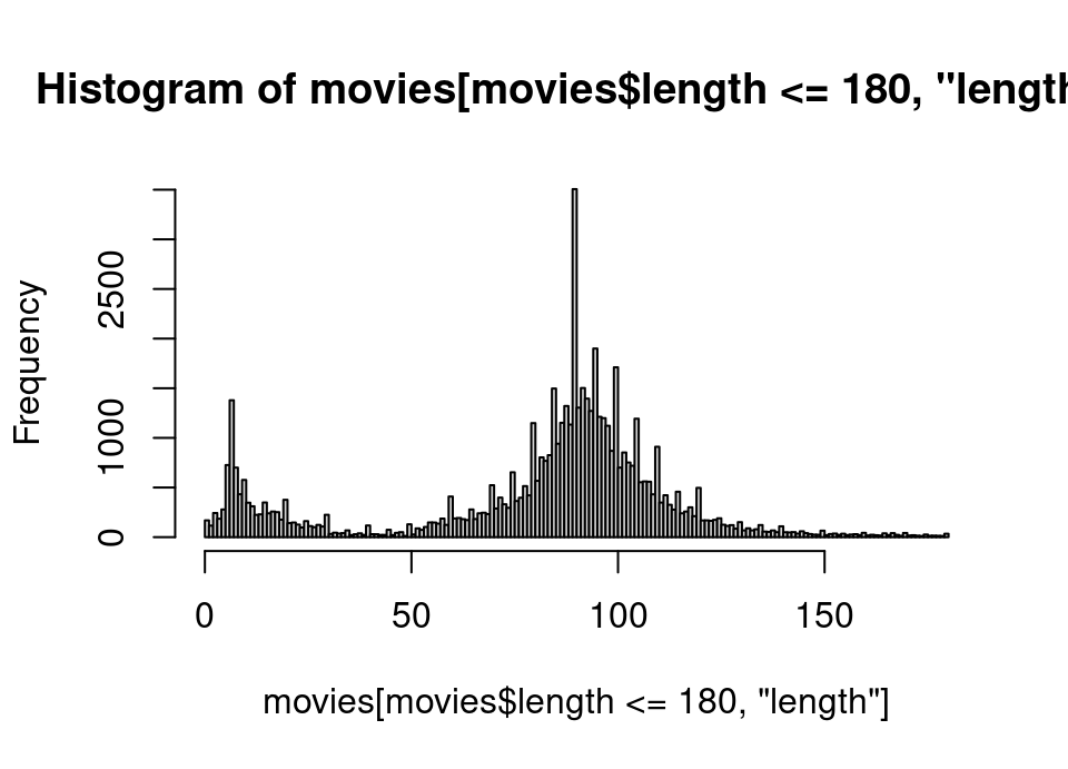
Exercise 5.50 Investigate for what histogram bin movie lengths these unusual patterns on the histogram appear.
In particular, by looking at the help file be sure to determine whether the histogram bins are left open or right open intervals. (ie are the bins \([x_1, x_2), [x_2, x_3), \dots\) or \((x_1, x_2], (x_2, x_3], \dots\)?)
Click for solution
We save the histogram object, just like we did in the lecture, so that we can examine the detail of the histogram:
## SOLUTION

h <- hist(movies[movies$length<=180,"length"], breaks = seq(0, 180, 1))
str(h)List of 6
$ breaks : num [1:181] 0 1 2 3 4 5 6 7 8 9 ...
$ counts : int [1:180] 169 116 243 185 279 726 1379 700 432 576 ...
$ density : num [1:180] 0.00289 0.00199 0.00416 0.00317 0.00478 ...
$ mids : num [1:180] 0.5 1.5 2.5 3.5 4.5 5.5 6.5 7.5 8.5 9.5 ...
$ xname : chr "movies[movies$length <= 180, \"length\"]"
$ equidist: logi TRUE
- attr(*, "class")= chr "histogram"Notice that h contains the list structure we saw in lectures.
We are interested in the $breaks and $counts variables.
The $breaks is 1 longer than $counts since it defines the boundaries of the bins, so for example the first count of 169 applies to the interval 0–1.
Let’s get the indices in descending order for the $count variable, which will correspondingly tell us the index in $breaks for the left end of the interval of the highest spikes on the histogram. We can then use perhaps the first 3 of these to get the movie length for the highest few spikes.
# NOTE: check the help file ?order and you'll see order sorts ascending by
# default! So we need to change to descending.
desc.length <- order(h$counts, decreasing = TRUE)
h$breaks[desc.length[1:3]]
[1] 89 94 99So we have these odd spikes in the intervals 89–90, 94–95, 99–100. The question also urges us to be certain about whether these are left or right open intervals. Look at the documentation:
?histExercise 5.51 Create a scatterplot of movie length against the year of release. Make sure to restrict the y-axis to the range 0–500 so that things are clearer.
Add to this a lowess smoother and straight line as shown in lectures. What might you conclude?
Click for solution
## SOLUTION
plot(movies$year, movies$length, ylim = c(0, 500))
lines(lowess(movies$year, movies$length), col = "red")
abline(lm(movies$length ~ movies$year), col = "green")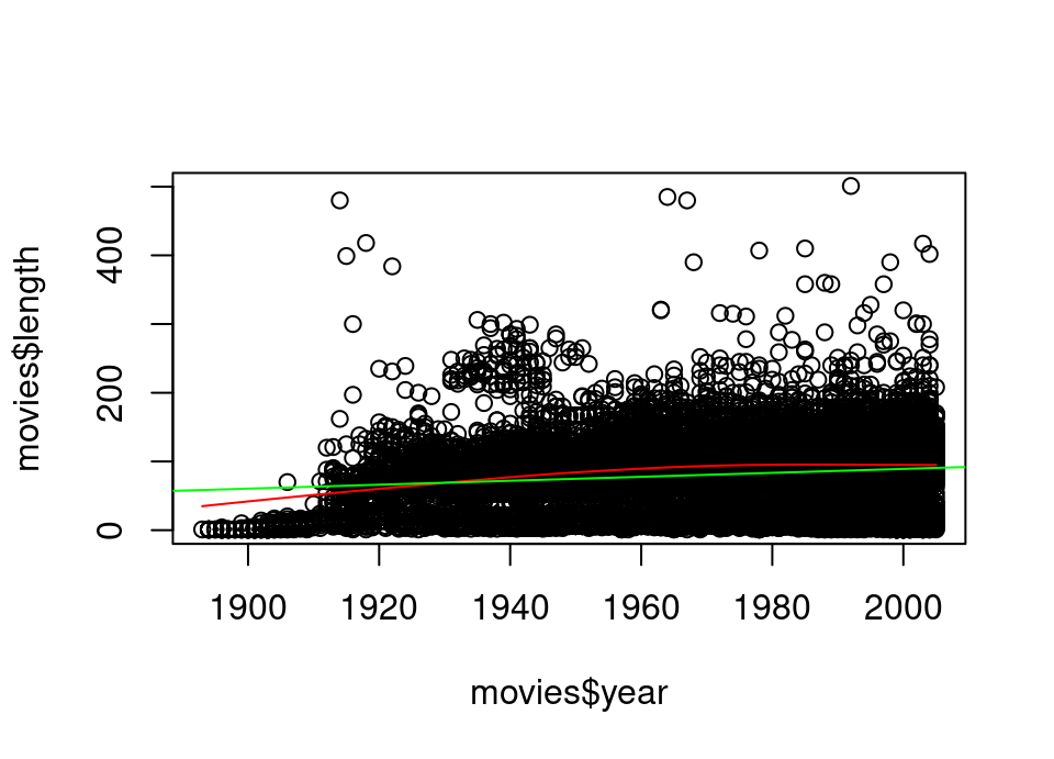 Both a smoother and straight line fit appear to show movies have been getting longer over the years. The smoother seems to indicate this trend may have ceased around 1980.
Exercise 5.52 (much longer, much harder, more fun!) You have not yet studied the mathematics of the lowess smoother or linear model, that fun is to come later in your degree! However, both models track the expectation (ie mean) of the y value, conditional on the value of x.
In order to check we are not observing an artefact of some of the massive movie lengths we saw earlier, let’s see how the median varies over the decades:
- Write a function which will take a vector of data and calculate the bootstrap confidence interval of the median of that data (using the method you’ve seen in tutorials this week)
- Write a for loop which will create a new data frame one row at a time for each decade in the data. It should have three variables: the decade, the lower, and the upper bootstrap confidence interval for the median. (Hint: the function
rbind()enables you to join two data frames together by rows, and if one of them isNULLyou just get the non-null data frame) - Draw a line plot showing the lower and upper 99% confidence interval for the median movie length for each decade. (Hint: see
plotfunction withtype = "l"andlinesfunction)
The solution is split in 3: do try and think very hard about each part before looking. Once you look, if it is not how you did it then work carefully through to understand how each small part works and ask for help if anything isn’t clear!
Click for solution (i)
bootstrap <- function(x, ci = 0.99, B = 10000) {
  S.star <- rep(0, B)
  for(i in 1:B) {
    x.star <- sample(x, replace = TRUE)
    S.star[i] <- median(x.star)
  }

  lower <- sort(S.star)[round((1-ci)/2*B)]
  upper <- sort(S.star)[round((ci+(1-ci)/2)*B)]

  return(c(lower, upper))
}
Click for solution (ii)
# By looking at:
range(movies$year)
[1] 1893 2005# we see that the decades in the data run from 1890/1900 to 2000/2010.
# Using the hint, we will create a NULL then rbind 1-row data frames to it
# to hold the median confidence intervals
med.CIs <- NULL
for(decade in seq(1890, 2000, 10)) {
new.CI <- bootstrap(movies[movies$year >= decade & movies$year < decade+10,"length"])
med.CIs <- rbind(med.CIs,
data.frame(decade = decade,
lower = new.CI[1],
upper = new.CI[2]))
}
# Now we should have the required data frame:
med.CIs decade lower upper
1 1890 1.0 1
2 1900 3.0 5
3 1910 19.0 31
4 1920 69.0 75
5 1930 69.0 71
6 1940 74.0 78
7 1950 84.5 86
8 1960 91.0 93
9 1970 93.0 94
10 1980 93.0 94
11 1990 92.0 93
12 2000 90.0 90Click for solution (iii)
# As explained in the lecture, we need to use plot first as this creates a new
# plot, so we will call with line type.
# Also we add 5 to centre the point in the middle of the decade
plot(med.CIs$decade+5, med.CIs$lower, type="l")
# Then we add the upper confidence interval by using lines to add to the plot
lines(med.CIs$decade+5, med.CIs$upper, type="l")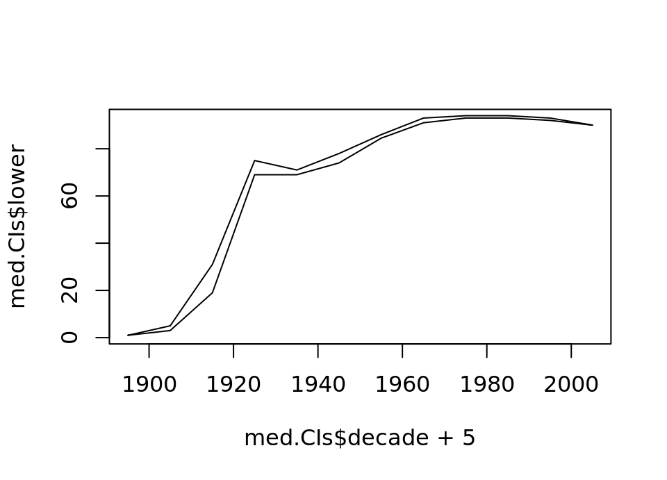 This is really nice: with so much data the confidence intervals on our bootstrap are really tight! It looks like median lengths have actually slightly reduced toward the end of the data set.
🏁🏁 Done, end of lab! 🏁🏁