Lab 10: Dates & Strings
🧑💻 Make sure to finish all previous labs before continuing with this one! It might be tempting to skip some stuff if you’re behind, but you may just end up progressively more lost … we will happily answer questions from any lab each week 😃
NOTE: with my enthusiasm for presenting Shiny, we got a little behind in the lecture, so if your lab takes place before Thursday in Week 10, then you won’t quite have seen everything for this lab.
I would recommend you continue through the first dates part, and get practice at looking at the lubridate package documentation (sometimes easier looking at the Reference page of the website https://lubridate.tidyverse.org/).
However, the second part on strings is comparatively complex, so I’d hold on to that for after the Thursday lecture to wrap up in your own time.
I (Louis, your lecturer) will be happy to answer any questions that arise from the later part because I realise this is the last supervised lab with me, Jochen, or Adam.
5.14 New York City flights 🛫
We’ll revisit the flights data to flex our new date manipulation skills, so make sure to load the Tidyverse, lubridate and the flight data:
library("tidyverse")
library("lubridate")

data("flights", package = "nycflights13")
Also remind yourself of the meaning of all the variables by looking at the help for this data:
?nycflights13::flightsExercise 5.94 Create two new variables, called sched_dep_hour and sched_dep_min, which split sched_dep_time into the hour of the day and minutes past the hour (these already exist with a different name in the data, but we want to practice!)
Then, create a new variable called sched_dep which uses year, month, day, sched_dep_hour and sched_dep_min to create a date-time representing when the flight was scheduled to depart.
Make sure this is set to the America/New_York time zone and once this new date-time variable exists, remove the sched_dep_hour and sched_dep_min variables: these we just required temporarily to get to the full date-time representation.
Click for solution
According to the documentation, sched_dep_time contains:
Scheduled departure and arrival times (format HHMM or HMM), local tz.
Therefore, to get the hour we would divide by 100 and round down with floor().
Then, to get the minutes, we would subtract \(100\times\) whatever we got for the hour.
All this is easily done inside a mutate() command (see dplyr from lecture practical/lab 5).
## SOLUTION

flights <- flights |>
  mutate(sched_dep_hour = floor(sched_dep_time/100),
         sched_dep_min = sched_dep_time - sched_dep_hour*100)
With this done, we can use the new function we learned this week, make_datetime(), and reference the other columns which contain the date (see docs: year, month, day).
Then, we can remove the temporary hour and minute calculations we did using the dplyr select.
## SOLUTION

flights <- flights |>
  mutate(sched_dep = make_datetime(year, month, day, sched_dep_hour, sched_dep_min, tz = "America/New_York")) |>
  select(-sched_dep_hour, -sched_dep_min)
Exercise 5.95 Summarise the average departure delay by day of the week for which the flight was scheduled.
Repeat the calculation, excluding negative delays (recall from the last lab, these were early flights).
Click for solution
## SOLUTION

flights |>
  mutate(day_of_week = wday(sched_dep, label = TRUE)) |>
  group_by(day_of_week) |>
  summarise(avg_delay = mean(dep_delay, na.rm = TRUE))
# A tibble: 7 × 2
day_of_week avg_delay
<ord> <dbl>
1 Sun 11.6
2 Mon 14.8
3 Tue 10.6
4 Wed 11.8
5 Thu 16.1
6 Fri 14.7
7 Sat 7.65flights |>
filter(dep_delay >= 0) |>
mutate(day_of_week = wday(sched_dep, label = TRUE)) |>
group_by(day_of_week) |>
summarise(avg_delay = mean(dep_delay, na.rm = TRUE))# A tibble: 7 × 2
day_of_week avg_delay
<ord> <dbl>
1 Sun 33.2
2 Mon 38.9
3 Tue 32.8
4 Wed 34.8
5 Thu 38.6
6 Fri 36.1
7 Sat 26.5Exercise 5.96 (Much Harder!!)
Continuing the last exercise: write your own function to calculate a bootstrap estimate of the standard error in the mean for the departure delay on each day of the week and so calculate a simple Normal confidence interval for the mean. Use 200 bootstrap simulations. Apart from the function which calculates the bootstrap standard error, everything else should be done within Tidyverse functions.
Then, by looking at the help file for geom_errorbarh in ggplot2, create a plot showing these confidence intervals for each day of the week.
Click for solution
## SOLUTION

# Function to perform bootstrap and return the standard error
bootstrap.se <- function(x) {
  B <- 200

  # Statistic
  S <- mean

  # Perform bootstrap
  S.star <- rep(0, B)
  for(b in 1:B) {
    x.star <- sample(x, replace = TRUE)
    S.star[b] <- S(x.star)
  }

  return(sd(S.star))
}

# Tidyverse pipeline adding calculation of the bootstrap standard error for
# each day of week grouping using above function, with a final mutate to
# compute confidence interval
mean_ci <- flights |>
  filter(dep_delay >= 0) |>
  mutate(day_of_week = wday(sched_dep, label = TRUE)) |>
  group_by(day_of_week) |>
  summarise(mean_delay = mean(dep_delay, na.rm = TRUE),
            bootstrap_se = bootstrap.se(dep_delay)) |>
  mutate(mean_ci_lower = mean_delay - 1.96*bootstrap_se,
         mean_ci_upper = mean_delay + 1.96*bootstrap_se)
mean_ci
# A tibble: 7 × 5
day_of_week mean_delay bootstrap_se mean_ci_lower mean_ci_upper
<ord> <dbl> <dbl> <dbl> <dbl>
1 Sun 33.2 0.360 32.5 33.9
2 Mon 38.9 0.377 38.2 39.7
3 Tue 32.8 0.327 32.2 33.5
4 Wed 34.8 0.360 34.1 35.5
5 Thu 38.6 0.367 37.9 39.3
6 Fri 36.1 0.340 35.5 36.8
7 Sat 26.5 0.362 25.8 27.2# Visualisation of the confidence interval of the mean delay
ggplot(mean_ci, aes(x = mean_delay, y = day_of_week)) +
geom_point() +
geom_errorbarh(aes(xmin = mean_ci_lower, xmax = mean_ci_upper))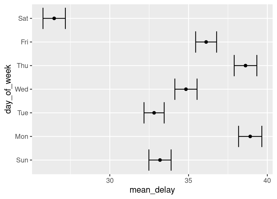
The package containing this flight data also contains weather data at an hourly resolution in the weather data frame.
data("weather", package = "nycflights13")You will see the final column, time_hour, is a date-time column where the minutes and seconds are zero indicating that this reading applies to the displayed hour.
Exercise 5.97 The flights data frame contains a column named time_hour to enable joining with the weather table.
If it wasn’t already there, how would you create the time_hour variable from the sched_dep variable you made earlier in the lab?
Click for solution
We’ll make a variable time_hour2 using the floor_date() function from the most recent lecture practical and then check it matches the time_hour variable.
## SOLUTION

flights <- flights |>
  mutate(time_hour2 = floor_date(sched_dep, unit = "hour"))

all(flights$time_hour == flights$time_hour2)
[1] TRUE5.15 Strings
The stringr package contains a dataset called sentences which is a standardised collection of sentences for testing voice.
data("sentences", package = "stringr")Exercise 5.98 What is the average length of each sentence?
What is the shortest and longest sentence?
Click for solution
## SOLUTION

mean(str_length(sentences))
[1] 39.35417sentences[which.min(str_length(sentences))][1] "Next Tuesday we must vote."sentences[which.max(str_length(sentences))][1] "The bills were mailed promptly on the tenth of the month."Exercise 5.99 Do any of the sentences contain extraneous whitespace anywhere within them?
Click for solution
To test this, we can str_squish() the strings and check if the length changes or not.
## SOLUTION

any(str_length(str_squish(sentences)) != str_length(sentences))
[1] FALSEExercise 5.100 What (if any) sentences are about sheep? 🐑
Click for solution
## SOLUTION

with_sheep <- str_detect(sentences, "sheep")

sentences[with_sheep]
[1] "Tend the sheep while the dog wanders."
[2] "The sheep were led home by a dog." Exercise 5.101 Are there any capital letters used except at the start of a sentence?.
Click for solution
## SOLUTION

with_caps <- str_detect(sentences, "^.+[A-Z]")

sentences[with_caps]
[1] "The Navy attacked the big task force."
[2] "A Tusk is used to make costly gifts."
[3] "Cats and Dogs each hate the other."
[4] "The wreck occurred by the bank on Main Street."
[5] "The map had an X that meant nothing."
[6] "The rush for funds reached its peak Tuesday."
[7] "Next Tuesday we must vote."
[8] "A cone costs five cents on Mondays."
[9] "He takes the oath of office each March."
[10] "The beetle droned in the hot June sun."
[11] "Next Sunday is the twelfth of the month."
[12] "The rarest spice comes from the far East."
[13] "A smatter of French is worse than none." Exercise 5.102 Extract any sentence containing a day of the week and replace each occurrence of a day with the three letter abbreviation of that day (ie “Sunday” \(\to\) “Sun”, “Monday” \(\to\) “Mon”, etc)
Hint: you will need to read the documentation for str_replace()!
Click for solution
The solution involving lots of typing is:
## SOLUTION

with_day <- str_detect(sentences, "Monday|Tuesday|Wednesday|Thursday|Friday|Saturday|Sunday")

day_sentence <- sentences[with_day]

str_replace_all(day_sentence, c("Monday"    = "Mon",
                                "Tuesday"   = "Tue",
                                "Wednesday" = "Wed",
                                "Thursday"  = "Thu",
                                "Friday"    = "Fri",
                                "Saturday"  = "Sat",
                                "Sunday"    = "Sun"))
[1] "Sun is the best part of the week."
[2] "The rush for funds reached its peak Tue."
[3] "Next Tue we must vote."
[4] "A cone costs five cents on Mons."
[5] "Next Sun is the twelfth of the month." There is a ‘clever’ solution which means only typing in the days of the week once:
dow <- c("Monday", "Tuesday", "Wednesday", "Thursday", "Friday", "Saturday", "Sunday")

dow_regex <- str_c(dow, collapse = "|")

with_day <- str_detect(sentences, dow_regex)

day_sentence <- sentences[with_day]

dow_replace <- str_sub(dow, 1, 3)
names(dow_replace) <- dow

str_replace_all(day_sentence, dow_replace)
[1] "Sun is the best part of the week."
[2] "The rush for funds reached its peak Tue."
[3] "Next Tue we must vote."
[4] "A cone costs five cents on Mons."
[5] "Next Sun is the twelfth of the month." 🏁🏁 Done, end of lab! 🏁🏁