Tutorial 4, Week 8 Solutions
Q1
(a)
If we have that \(X \sim \text{Exp}(\lambda=1)\), then using the hint, we can see that the integral is simply:
\[\begin{align*} \mu = \int_0^1 x \lambda e^{-\lambda x} \, dx &= \int_0^1 x f_X(x) \, dx \\ &= \int_{\mathbb{R}} x\ \bbone\{ x \in [0,1] \} f_X(x) \, dx \\ &= \mathbb{E}\left[X\ \bbone\{ X \in [0,1] \}\right] \end{align*}\]
(b)
Using integration by parts, \[\begin{align*} u &= x, & dv &= e^{-x} \\ du &= 1, & v &= -e^{-x} \end{align*}\]
\[\begin{align*} \int x e^{-x} \, dx &= -x e^{-x} + \int e^{-x}\,dx \\ &= -e^{-x} (1 + x) \\ \implies \int_0^1 x e^{-x} \, dx &= \left[ -e^{-x} (1 + x) \right]_0^1 \\ &= -e^{-1} (1 + 1) + e^{-0} (1 + 0) \\ &= 1 - 2e^{-1} \\ &\approx 0.2642 \end{align*}\]
Therefore, \(\mathbb{E}\left[X\ \bbone\{ X \in [0,1] \}\right] = 1 - 2e^{-1} \approx 0.2642\).
(c)
- Simulate \(x_1, \dots, x_n\) from an Exponential(\(\lambda=1\)) distribution
- Calculate \[\hat{\mu}_n = \frac{1}{n} \sum_{i=1}^n x_i\ \bbone\{ x_i \in [0,1] \}\]
(d)
We know from lectures that \[\text{Var}\left(\hat{\mu}_n\right) = \mathbb{E}\left[(\hat{\mu}_n - \mu)^2\right] = \frac{\sigma^2}{n}\] where here we have \[\sigma^2 = \text{Var}\left(X\ \bbone\{ X \in [0,1] \}\right)\] with \(X \sim \text{Exp}(\lambda=1)\).
Based on the hint, we want to find: \[\text{Var}\left(X\ \bbone\{ X \in [0,1] \}\right) = \mathbb{E}\left[ \left(X\ \bbone\{ X \in [0,1] \} \right)^2\right] - \mathbb{E}\left[X\ \bbone\{ X \in [0,1] \}\right]^2\]
We already know from (b) that \(\mathbb{E}\left[X\ \bbone\{ X \in [0,1] \}\right] = 1 - 2e^{-1}\), so we just need:
\[\begin{align*} \mathbb{E}\left[\left(X\ \bbone\{ X \in [0,1] \}\right)^2\right] &= \int_{\mathbb{R}} \left( x\ \bbone\{ x \in [0,1] \} \right)^2 f_X(x) \, dx \\ &= \int_0^1 x^2 e^{-x} \, dx \end{align*}\]
Again, a simple application of integration by parts gives:
\[\begin{align*} \int x^2 e^{-x} \, dx &= -x^2 e^{-x} - \int -2x e^{-x} \,dx \\ &= -x^2 e^{-x} + 2 \int x e^{-x} \,dx \end{align*}\]
We know the remaining integral from (b), so we get:
\[\begin{align*} \int x^2 e^{-x} \, dx &= -x^2 e^{-x} + 2 \left( -e^{-x} (1 + x) \right) \\ \implies \int_0^1 x^2 e^{-x} \, dx &= \left[ - e^{-x} (2 + 2x + x^2) \right]_0^1 \\ &= -e^{-1} (2 + 2 + 1) + e^{0} (2 + 0 + 0) \\ &= 2 - 5e^{-1} \\ &\approx 0.1606 \end{align*}\]
So,
\[\begin{align*} \text{Var}\left(X\ \bbone\{ X \in [0,1] \}\right) &= \underbrace{(2 - 5e^{-1})}_{\mathbb{E}\left[ \left(X\ \bbone\{ X \in [0,1] \} \right)^2\right]} - \underbrace{(1 - 2e^{-1})^2}_{\mathbb{E}\left[X\ \bbone\{ X \in [0,1] \}\right]^2} \\ &= 1 - e^{-1} - 4 e^{-2} \\ &\approx 0.09078 \end{align*}\]
Thus, \[\text{Var}\left(\hat{\mu}_n\right) \approx \frac{0.09078}{n}\]
Q2
(a)
Let \(X\) have Uniform distribution on \([0,1]\), so that: \[f_X(x) = \begin{cases} 1 & \text{if } x \in [0,1] \\ 0 & \text{otherwise}\end{cases}\]
Then, \[\begin{align*} \mu = \int_0^1 x e^{-x} \, dx &= \int_0^1 x e^{-x} f_X(x) \, dx \\ &= \int_{\mathbb{R}} x e^{-x} f_X(x) \, dx \\ &= \mathbb{E}\left[X e^{-X}\right] \end{align*}\]
(b)
- Simulate \(x_1, \dots, x_n\) from a Uniform(0, 1) distribution
- Calculate \[\hat{\mu}_n = \frac{1}{n} \sum_{i=1}^n x_i e^{-x_i}\]
(c)
As for Q1(d), we know from lectures that \[\text{Var}\left(\hat{\mu}_n\right) = \mathbb{E}\left[(\hat{\mu}_n - \mu)^2\right] = \frac{\sigma^2}{n}\] However, now \[\sigma^2 = \text{Var}\left(X e^{-X}\right)\] with \(X \sim \text{Unif}(0,1)\).
We will again use the standard formula for the variance:
\[\text{Var}\left(X e^{-X}\right) = \mathbb{E}\left[ \left(X e^{-X}\right)^2 \right] - \mathbb{E}\left[ X e^{-X} \right]^2\]
We know that Monte Carlo integration is unbiased, so the second term is unchanged in value despite the different problem formulation,
\[\mathbb{E}\left[ X e^{-X} \right] = 1 - 2e^{-1} \approx 0.2642\]
So we just need:
\[\begin{align*} \mathbb{E}\left[ \left(X e^{-X}\right)^2 \right] &= \int x^2 e^{-2x} f_X(x) \,dx \\ &= \int_0^1 x^2 e^{-2x} \,dx \end{align*}\]
Using the hint in the question to save time on integration, we find:
\[\begin{align*} \int_0^1 x^2 e^{-2x} \,dx &= \left[ -\frac{e^{-2x}}{4} (2x^2 + 2x + 1) \right]_0^1 \\ &= - \frac{5}{4} e^{-2} + \frac{1}{4} \\ &\approx 0.08083 \end{align*}\]
Therefore,
\[\begin{align*} \text{Var}\left(X e^{-X}\right) &= \underbrace{\frac{1}{4} - \frac{5}{4} e^{-2}}_{\mathbb{E}\left[ \left(X e^{-X}\right)^2 \right]} - \underbrace{\left(1 - 2e^{-1}\right)^2}_{\mathbb{E}\left[ X e^{-X} \right]^2} \\ &= 4 e^{-1} - \frac{21}{4} e^{-2} -\frac{3}{4} \\ &\approx 0.01101 \end{align*}\]
Thus, \[\text{Var}\left(\hat{\mu}_n\right) \approx \frac{0.01101}{n}\]
(d)
The width of the confidence interval for Monte Carlo integration is \[z_{\alpha/2} \frac{\sigma}{\sqrt{n}}\]
Letting \(\sigma_E^2\) and \(n_E\) be the variance and simulation size under Exponential sampling, and \(\sigma_U^2\) and \(n_U\) be the variance and simulation size under Uniform sampling, we would need: \[\begin{align*} z_{\alpha/2} \frac{\sigma_E}{\sqrt{n_E}} &= z_{\alpha/2} \frac{\sigma_U}{\sqrt{n_U}} \\ \implies \frac{n_E}{n_U} &= \frac{\sigma_E^2}{\sigma_U^2} \\ \implies \frac{n_E}{n_U} &= \frac{0.09078}{0.01101} = 8.25 \end{align*}\]
So we would need to take \(8.25\times\) times as many simulations from an Exponential to achieve the same accuracy as using Uniform simulations!
Q3
(a)
Given the probability density function in the question, we need to find the cdf:
\[F_X(x) = \int_{-\infty}^x \alpha z^{\alpha-1} \, dz = \begin{cases} 0 & \text{if } x < 0 \\ x^\alpha & \text{if } x \in [0,1] \\ 1 & \text{if } x > 1 \end{cases}\]
For example,
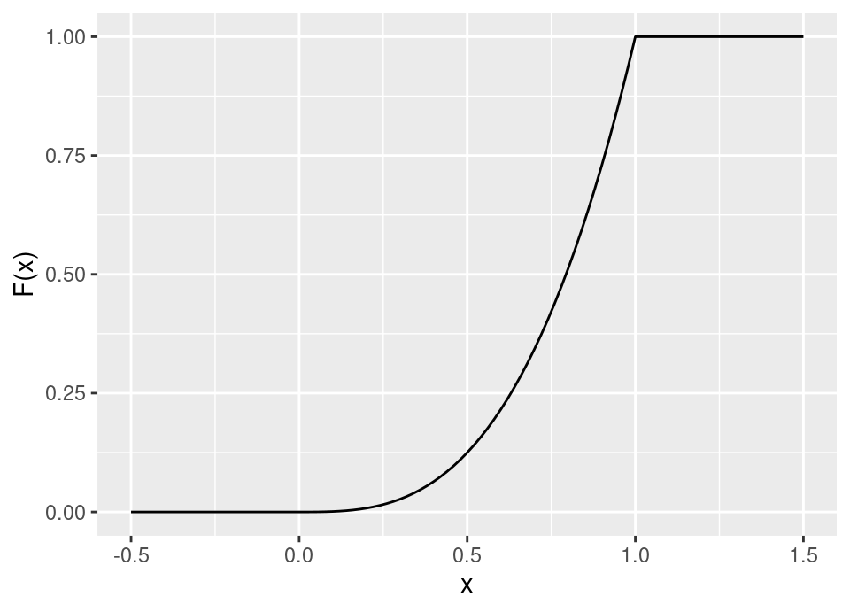
Therefore, \(F^{-1}(u) = u^{\frac{1}{\alpha}}\).
Hence, we simulate from this probability density function by simulating \(U \sim \text{Unif}(0,1)\) and then return \(X = u^{\frac{1}{\alpha}}\).
(b)
Let \(X\) have probability density function \(f_X(x)\) as given in the question, \[\begin{align*} \mu = \int_0^1 x e^{-x} \, dx &= \int_0^1 \frac{1}{f_X(x)} x e^{-x} f_X(x) \, dx \\ &= \int_{\mathbb{R}} \alpha^{-1} x^{-\alpha+1} x e^{-x} f_X(x) \, dx \\ &= \int_{\mathbb{R}} \alpha^{-1} x^{-\alpha+2} e^{-x} f_X(x) \, dx \\ &= \mathbb{E}\left[\alpha^{-1} x^{-\alpha+2} e^{-x}\right] \end{align*}\]
(c)
- Simulate \(x_1, \dots, x_n\) from the pdf given in the question, perhaps using inverse sampling as described in (a)
- Calculate \[\hat{\mu}_n = \frac{1}{n} \sum_{i=1}^n \alpha^{-1} x^{-\alpha+2} e^{-x}\]
(d)
As for Q1(d) & Q2(c), we know from lectures that \[\text{Var}\left(\hat{\mu}_n\right) = \mathbb{E}\left[(\hat{\mu}_n - \mu)^2\right] = \frac{\sigma^2}{n}\] However, now \[\sigma^2 = \text{Var}\left(\alpha^{-1} x^{-\alpha+2} e^{-x}\right)\] with \(X\) simulated from \(f_X(\cdot)\).
We are told \(\alpha=2\), so we want:
\[\text{Var}\left(0.5 e^{-X}\right) = \mathbb{E}\left[ \left(0.5 e^{-X}\right)^2 \right] - \mathbb{E}\left[ 0.5 e^{-X} \right]^2\]
We know that Monte Carlo integration is unbiased, so the second term is unchanged in value despite the different problem formulation,
\[\mathbb{E}\left[ 0.5 e^{-X} \right] = 1 - 2e^{-1} \approx 0.2642\]
So we just need:
\[\begin{align*} \mathbb{E}\left[ \left(0.5 e^{-X}\right)^2 \right] &= \int 0.25 e^{-2x} f_X(x) \,dx \\ &= \int_0^1 0.25 e^{-2x} \times 2 x \,dx \\ &= 0.5 \int_0^1 x e^{-2x} \,dx \\ &= 0.5 \left[ -\frac{e^{-2x}}{4} (2x + 1) \right]_0^1 & \text{using hint} \\ &= \frac{1}{8} - \frac{3}{8} e^{-2} \\ &\approx 0.07425 \end{align*}\]
Therefore,
\[\begin{align*} \text{Var}\left(0.5 e^{-X}\right) &= \underbrace{\frac{1}{8} - \frac{3}{8} e^{-2}}_{\mathbb{E}\left[ \left(0.5 e^{-X}\right)^2 \right]} - \underbrace{\left(1 - 2e^{-1}\right)^2}_{\mathbb{E}\left[ 0.5 e^{-X} \right]^2} \\ &= 4 e^{-1} - \frac{35}{8} e^{-2} - \frac{7}{8} \\ &\approx 0.004426 \end{align*}\]
Thus, \[\text{Var}\left(\hat{\mu}_n\right) \approx \frac{0.004426}{n}\]
(e)
The logic is as for Q2(d). So,
\[\frac{0.09078}{0.004426} = 20.51\]
So we would need more than \(20\times\) as many simulations from an Exponential to achieve the same accuracy.
\[\frac{0.01101}{0.004426} = 2.49\]
So we would need \(2.49\times\) as many simulations from a Uniform to achieve the same accuracy.