Chapter 4 Monte Carlo Integration
⏪ ⏩
We have now seen simulation used to perform hypothesis testing, and estimation of uncertainty through the standard error and confidence intervals. There is one more very important area to cover in how simulation methods can be used, before we then spend the remainder of the course explaining how we handle simulation from arbitrary probability distributions. That topic is Monte Carlo Integration.
4.1 Motivating example: estimating \(\pi\) by simulation3
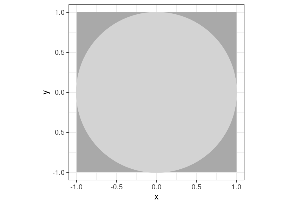
We know from the dim and distant past at school that the area of the above circle is \(\pi\), but let’s imagine for now that we don’t know the actual value for \(\pi\). However, assume we can select \((x,y)\) coordinates uniformly at random from the \(1\times1\) square containing the circle (uniformly at random just means that every possible coordinate \((x,y), x \in [-1,1], y \in [-1,1]\) is equally likely). This can be achieved if I can simulate two iid values \(X, Y \sim \text{Unif}(-1,1)\) from a uniform distribution on the interval \([-1,1]\).
What is the probability that any randomly sampled coordinate I select will fall inside the light grey circle, rather than in the dark grey corners?
\[\begin{align*} \mathbb{P}(\text{sampled coordinates inside circle}) &= \frac{\int \int_{\{x^2+y^2 \le 1\}} 1 \,dx\,dy}{\int_{-1}^1 \int_{-1}^1 1 \,dx\,dy} \\ &= \frac{\pi}{4} \\ \implies \pi &= 4 \times \mathbb{P}(\text{sampled coordinates inside circle}) \end{align*}\]
So, if we knew the probability we could compute \(\pi\). We can use simulation to tackle this by performing a simulation experiment which will sample many coordinates and examine the proportion inside the circle. How is this justified? Well, if I perform \(n\) simulations of this experiment, then the total number falling inside the circle, \(m\), will be Binomially distributed, \(M \sim \text{Bin}(n, p)\) where \(p = \mathbb{P}(\text{sampled coordinates inside circle})\).
So, we can estimate (Stats I) \(\hat{p} = \frac{m}{n}\) which leads to estimating \(\hat{\pi} = \frac{4m}{n}\). Let’s do it! …
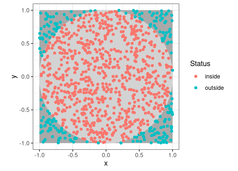
The above experiment is 2000 samples from a uniform distribution between -1 and 1, with 1000 used as x coordinates and 1000 as y coordinates, for a total of 1000 points. In total we got 770 falling inside the circle, so we estimate \(\hat{p}=0.77\), leading to an estimate \(\hat{\pi}=3.08\).
Try for yourself:
n <- 1000

x <- runif(n, -1, 1)
y <- runif(n, -1, 1)

inside <- (x^2+y^2 <= 1)
m <- sum(inside)

plot(x, y,
     pch = ifelse(x^2+y^2 <= 1, 20, 1),
     col = ifelse(x^2+y^2 <= 1, "green", "red"),
     cex = 0.5,
     asp = 1, xlim = c(-1, 1), ylim = c(-1, 1))
xx <- seq(-1, 1, len = 200)
lines(xx, sqrt(1-xx^2))
lines(xx, -sqrt(1-xx^2))

cat("Estimate of pi:", 4*m/n)
So after 1000 simulations, we’re still not getting a brilliant estimate, but fortunately we know (Prob I) that the (strong) law of large numbers ensures that \(\hat{\pi} = \frac{4M}{n} \to \pi\) as \(n \to \infty\). Until we have infinite compute power, we may have to make do with a good old fashioned Binomial confidence interval (Stats I) … with 95% confidence we have an interval for \(p\) of: \[\hat{p} \pm 1.96 \sqrt{\frac{\hat{p}(1-\hat{p})}{n}} = 0.77 \pm 1.96 \sqrt{\frac{0.77(1-0.77)}{1000}} = [0.7439165, 0.7960835]\] leading to an interval for \(\pi\) of quadruple this: \[[2.9756661, 3.1843339]\]
🤔 But, doesn’t that mean I could perhaps integrate any function over a finite range without knowing any calculus, as long as I can evaluate the function?
Pretty much, yes!
But we don’t want to do this in an ad-hoc manner for every problem, so we’ll abstract this and understand what the general formulation is that allows the above to work.
4.2 Monte Carlo Integration
Let us take it that the integral we want to evaluate can be expressed as an expectation for some random variable \(Y\) taking values in a sample space \(\Omega\) and having pdf \(f_Y(\cdot)\), then: \[\mu := \mathbb{E}[Y] = \int_\Omega y f_Y(y)\,dy\] If we assume \(\mu\) exists, we can approximate it by: \[\mu \approx \hat{\mu}_n := \frac{1}{n} \sum_{i=1}^n Y_i\] where \(Y_1, \dots, Y_n\) are iid draws from the distribution of \(Y\). Then, by the weak law of large numbers (Prob I): \[\lim_{n \to \infty} \mathbb{P}(| \hat{\mu}_n - \mu | \le \epsilon) = 1\] ie the probability that our approximation of the integral is out by more than \(\epsilon\) goes to zero. In fact, there is a strong law of large numbers too (which you won’t have seen in Prob I) which guarantees that at some point (as \(n\) increases) our error will drop below \(\epsilon\) and not increase: \[\mathbb{P}\left( \lim_{n \to \infty} | \hat{\mu}_n - \mu | = 0 \right) = 1\]
Important note: Never lose sight of the fact that \(\hat{\mu}_n\) is itself a random variable … it is a sum of random variables \(Y_i\), so is random!
Practically speaking, only evaluating integrals of the form: \[\mu := \mathbb{E}[Y] = \int_\Omega y f_Y(y)\,dy\] might seem limiting, but we will often find that we can express \(Y = g(X)\), where \(X\) is a random variable having pdf \(f_X(\cdot)\), so that: \[\mu := \mathbb{E}[Y] = \mathbb{E}[g(X)] = \int g(x) f_X(x)\,dx\]
Example 4.1 (Tackle 🥧 directly) Consider tackling the \(\pi\) problem above directly as a single integral in the setting just described. In other words, we must come up with a way to express the integral for \(\pi\) as an expectation of a random variable. We derive the solution above without making a geometric argument about areas, but by simply transforming the integral we are interested in to one we can estimate by Monte Carlo. We are really interested in the integral which was in the numerator before: \[\mu = \int \int_{\{x_1^2+x_2^2 \le 1\}} 1 \,dx_1\,dx_2 = \pi\] To simplify the limits of the integral and therefore simplify the space on which we must define a random variable, we can write: \[\mu = \int_{-1}^1 \int_{-1}^1 \bbone \{ x_1^2 + x_2^2 \le 1 \} \,dx_1\,dx_2\] The above form is not yet an expectation of a random variable though.
Given the region of integration is \([-1,1]\times[-1,1] \subset \mathbb{R}^2\), the simplest distribution we could use is Uniform on the whole square (as before). So, \(\vec{X}=(X_1,X_2)\) where, \[f_{\vec{X}}(\mathbf{x}) = f_{X_1}(x_1) f_{X_2}(x_2) = \begin{cases} \frac{1}{2} \times \frac{1}{2} & \text{ if } (x_1, x_2) \in [-1,1]\times[-1,1] \\ 0 & \text{ otherwise} \end{cases}\] Then, \[\begin{align*} \mu &= \int_{-1}^1 \int_{-1}^1 \bbone \{ x_1^2 + x_2^2 \le 1 \} \,dx_1\,dx_2 \\ &= \int_{-1}^1 \int_{-1}^1 \underbrace{4 \bbone \{ x_1^2 + x_2^2 \le 1 \}}_{g(\vec{x})} \times \underbrace{\frac{1}{4}}_{f_{\vec{X}}(\vec{x})} \,dx_1\,dx_2 \\ &= \iint_{\mathbb{R}^2} 4 \bbone \{ x_1^2 + x_2^2 \le 1 \} f_{\vec{X}}(x_1, x_2) \,dx_1\,dx_2 \\ &= \mathbb{E}\left[4 \bbone\{ X_1^2 + X_2^2 \le 1 \}\right] \end{align*}\]
Thus, we can simulate \(n\) samples \(x_{11}, \dots, x_{1n} \sim \text{Unif}(-1,1)\) and \(x_{21}, \dots, x_{2n} \sim \text{Unif}(-1,1)\) and calculate: \[\hat{\mu} = \frac{1}{n} \sum_{i=1}^n 4 \bbone\{ x_{1i}^2 + x_{2i}^2 \le 1 \}\]
Note this is exactly the same as the estimator we got by making the argument geometrically in terms of a ratio of two areas, but instead by directly tackling the exact integral of interest (the one in the numerator previously).
It’s not all about indicator functions, to avoid that misaprehension, let’s consider a super simple example where the indicator does not crop up:
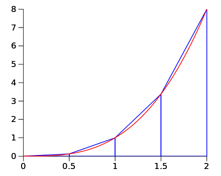
Example 4.2 (Kindergarden integration) Imagine we don’t even know how to compute the integral: \[\mu = \int_a^b x^2 \,dx\] Then, to do Monte Carlo integration without needing calculus, we could consider the random variable \(X \sim \text{Unif}(a, b)\), which has pdf: \[f_X(x) = \begin{cases} \frac{1}{b-a} & \text{ if } x \in [a,b] \\ 0 & \text{ otherwise} \end{cases}\] We then write: \[\mu = \int_a^b \underbrace{(b-a) x^2}_{g(x)} \underbrace{\frac{1}{b-a}}_{f_X(x)} \,dx = \int_\mathbb{R} (b-a) x^2 f_X(x)\,dx = \mathbb{E}[(b-a) X^2]\]
# Change a, b and n to see how it does
a <- -0.5
b <- 1
n <- 100000

x <- runif(n, a, b)

# Monte Carlo integral estimate:
mean((b-a)*x^2)

# Exact integral value:
b^3/3-a^3/3

# Plot how the estimate varies with n
# Dashed line is exact answer
# This code is a little more complicated to make
# plotting fast even for large n
i <- round(seq(100, n, length.out = 1000))
#mc <- sapply(i, function(i) { mean((b-a)*x[1:i]) })
plot(i, cumsum((b-a)*x^2)[i]/i, type="l", xlab = "n", ylab = "Monte Carlo estimate")
abline(h = b^3/3-a^3/3, lty = 2)
Rather less kindergarden! … \[\begin{align*} \mu &= \int_0^\pi \sqrt{x^3 + \sqrt{x}}-x^2 \sin(4x) \,dx \\ &= \int_0^\pi \underbrace{\pi \left( \sqrt{x^3 + \sqrt{x}}-x^2 \sin(4x) \right)}_{g(x)} \underbrace{\frac{1}{\pi}}_{f_X(x)} \,dx \end{align*}\]
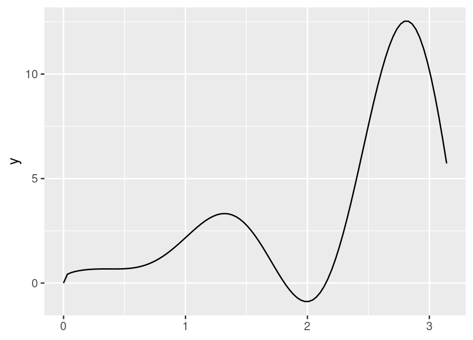
The exact answer is: \[\mu = \frac{\pi^2}{4} + \frac{2}{5}\left( \pi^{\frac{5}{4}} \sqrt{1+\pi^{\frac{5}{2}}} + \sinh^{-1}\left(\pi^{\frac{5}{4}}\right) \right)\]
# Change a, b and n to see how it does
n <- 100000

x <- runif(n, 0, pi)

# Monte Carlo integral estimate:
mean(pi * (sqrt(x^3 + sqrt(x))-x^2*sin(4*x)))

# Exact integral value:
pi^2/4 + 0.4*(pi^(5/4)*sqrt(1+pi^(5/2))+asinh(pi^(5/4)))

# Plot how the estimate varies with n
# Dashed line is exact answer
# This code is a little more complicated to make
# plotting fast even for large n
i <- round(seq(100, n, length.out = 1000))
#mc <- sapply(i, function(i) { mean((b-a)*x[1:i]) })
plot(i, cumsum(pi * (sqrt(x^3 + sqrt(x))-x^2*sin(4*x)))[i]/i, type="l", xlab = "n", ylab = "Monte Carlo estimate")
abline(h = pi^2/4 + 0.4*(pi^(5/4)*sqrt(1+pi^(5/2))+asinh(pi^(5/4))), lty = 2)
Probably get the idea! …
So in these toy examples, we’ve seen handling a general function and handling complex limits through indicators, and of course these ideas can be combined.
Note that the above setting (ie some simple deterministic function) is not the most common use case for Monte Carlo integration, but it provides an easy to understand motivation. In practice, the most common uses for Monte Carlo integration are statistical: computing expectations, probabilities and Bayesian posteriors.
4.2.1 Accuracy
If we further know that \(\text{Var}(Y) = \sigma^2 < \infty\), then we also have that: \[\mathbb{E}[\hat{\mu}_n] = \frac{1}{n} \sum_{i=1}^n \mathbb{E}[Y_i] = \mu\] In other words, Monte Carlo integration is unbiased. Further, we have that \[\text{Var}(\hat{\mu}_n) = \mathbb{E}[(\hat{\mu}_n - \mu)^2] = \frac{\sigma^2}{n}\] This is a result you’ve seen before for the mean so we don’t prove it again.
So the mean square error is \(\sigma^2/n\), though we often instead think about the root-mean square error which is on the same scale as the integral we’re estimating. \[\text{RMSE} := \sqrt{\mathbb{E}[(\hat{\mu}_n - \mu)^2]} = \frac{\sigma}{\sqrt{n}}\]
Notice that in this simple setting, \(\sigma^2\) is defined by the problem setup (since it is \(\text{Var}(Y)\)), so the main thing we can control is \(n\). Therefore, we say that the RMSE is \(\mathcal{O}(n^{-1/2})\) (spoken “is order n to the minus a half”).
Definition 4.1 (Order) For functions \(f\) and \(g\), we write that \(f(n) = \mathcal{O}(g(n))\) as \(n \to \infty\) if \(\exists\) \(C, n_0 \in \mathbb{R}\) st \(|f(n)| \le C g(n) \ \ \forall\, n \ge n_0\).
Order notation is useful for focusing on the rate at which a function converges without worrying about the specific constants \(C\) and \(n_0\).
What does an RMSE which is \(\mathcal{O}(n^{-1/2})\) mean practically? Well,
- to halve our error will require quadrupling the number of simulations we do (\(4^{-1/2} = \frac{1}{2}\));
- to get a full decimal place extra accuracy – a ten-fold increase in accuracy – requires 100\(\times\) the amount of simulation; etc.
- to get 5 more decimal places of accuracy requires 10,000,000,000\(\times\) the amount of simulation(!)
We’ll probably want to understand more sophisticated options in due course!
4.2.2 Numerical integration
You may reasonably be wondering why we go to the trouble of expressing an integral as an expectation when we could just do numerical integration, such as the midpoint Riemann sum, trapezoidal rule, or Simpson’s rule.
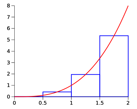
For example, the midpoint Riemann integral in the simple 1 dimensional setting using \(n\) evaluations is given by: \[\int_a^b g(x)\,dx \approx \frac{b-a}{n} \sum_{i=1}^n g(x_j)\] where \[x_i := a + \frac{b-a}{n}\left( j - \frac{1}{2} \right)\] Notice the striking similarity! Basically, if you use a Uniform distribution as \(f_X(\cdot)\), then the sum looks identical with the only difference being how to specify \(x_i\) … the Riemann sum does a regular grid and Monte Carlo simulates randomly.
It is possible to prove the absolute error in using the midpoint Riemann rule is bounded as: \[\left| \int_a^b g(x)\,dx - \frac{b-a}{n} \sum_{j=1}^n g(x_j) \right| \le \frac{(b-a)^3}{24 n^2} \max_{a \le z \le b} | g''(z)|\] Clearly, \(\frac{(b-a)^3}{24} \max_{a \le z \le b} | g''(z)|\) is fixed by integral we want to find and cannot be affected by the us, so we achieve the accuracy we require by controlling \(n^{-2}\) — that is, by using a finer grid to compute the integral. So, the error in the midpoint Riemann integral in 1 dimension is \(\mathcal{O}\left(n^{-2}\right)\). This is much better than Monte Carlo actually! To double the accuracy you only need to take \(\sqrt{2}\times\) more grid points, not \(4\times\) more simulations as for Monte Carlo.
BUT (you knew there was a “but” coming, right?!), as the dimension of \(x\) increases, the Riemann integral’s effectiveness diminishes fast. In general, the error of midpoint Riemann integration in \(d\)-dimensions is \(\mathcal{O}\left(n^{-2/d}\right)\). It is beyond our scope, but similarly more advanced numerical integration methods suffer the same dimensionality fate.
What about Monte Carlo? The striking thing is that for a \(d\)-dimensional problem, the RMSE is still \(\mathcal{O}\left(n^{-1/2}\right)\) … no \(d\) in sight!4 We see the differences illustrated below.
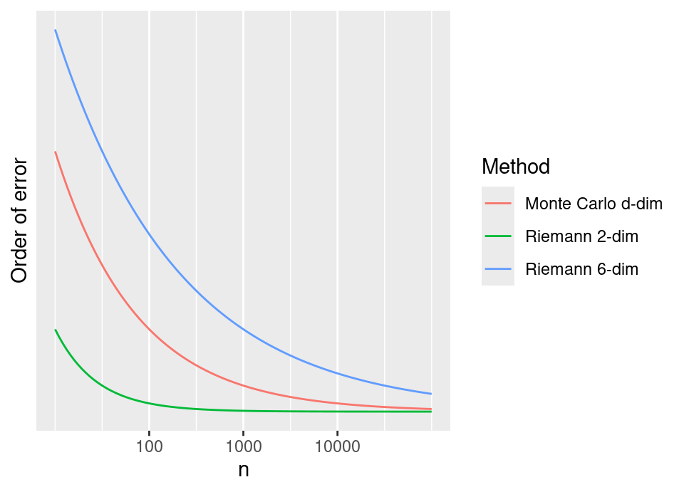
This shows the order of error reduction – that is, only the leading \(\mathcal{O}\left(n^{f(d)}\right)\) term – plotted against different computational effort \(n\). Note that all these curves would be multiplied by a different (fixed) problem dependent constant.
4.2.3 Error estimation
Another very nice property of Monte Carlo is that we can get an estimate of how accurate our integral approximation is for “free”, using the same simulations we used for calculating the integral (unlike standard numerical integration).
There are at least two options.
Firstly, we can use a simple application of Chebyshev’s inequality to provide a probabilistic bound on the absolute error exceeding a desired tolerance: \[\mathbb{P}(|\hat\mu_n - \mu| \ge \varepsilon) \le \frac{\mathbb{E}[(\hat\mu_n - \mu)^2]}{\varepsilon^2} = \frac{\sigma^2}{n \varepsilon^2}\]
Secondly, we can invoke the iid Central Limit Theorem (CLT) so that asymptotically, \[\mathbb{P}\left( \frac{\hat\mu - \mu}{\sigma n^{-1/2}} \le z \right) \xrightarrow{n\to\infty} \Phi(z)\] where \(\Phi(z)\) denotes the standard Normal cumulative distribution function (cdf). This enables the formation of familiar confidence intervals for \(\mu\),
Important note: We can be very happy using the CLT, because we know (and control!) \(n\) … it will definitely be large and we can ensure we are well into CLT territory, because we get to choose how big \(n\) is when we simulate! This is quite unlike most other places you have probably seen the CLT used in statistics, where it is often borderline and we might worry if \(n\) is big enough or not.
So, we can be \(100(1-\alpha)\)% confident that: \[\mu \in \hat{\mu}_n \pm z_{\alpha/2} \frac{\sigma}{\sqrt{n}}\] where \(\sigma\) is estimated using the standard sample standard deviation of \(\{ y_i=g(x_i) \}_{i=1}^n\).
Let’s confirm this by doing an experiment to see how often this confidence interval covers the true value of the integral for our moderatly complicated 1-dimensional integral example earlier:
# n is number of MC simulations for a single run
# runs is number of full MC estimators to calculate to check confidence interval
n <- 1000
runs <- 10000

# Exact integral value:
exact <- pi^2/4 + 0.4*(pi^(5/4)*sqrt(1+pi^(5/2))+asinh(pi^(5/4)))

in.ci <- 0
for(run in 1:runs) {
  x <- runif(n, 0, pi)
  g <- pi * (sqrt(x^3 + sqrt(x))-x^2*sin(4*x))

  mean.g <- mean(g)
  sd.g <- sd(g)

  if(exact >= mean.g - 1.96*sd.g/sqrt(n) & exact <= mean.g + 1.96*sd.g/sqrt(n)) {
    in.ci <- in.ci + 1
  }
}

# Percentage of times exact was inside the confidence interval
in.ci / runs * 100
You should see it is pretty much spot on 95%, showing the confidence interval is indeed excellently calibrated.
There is only one other confidence interval we’ll be interested in, which is the special case where \(g(\cdot)\) is some constant multiple of an indicator function (as we have for estimating \(\pi\), for example, and \(\sqrt{2}\) in tutorials), \[g(x) = c \bbone\{A(x)\}\] for some condition \(A(x)\) depending on \(x\) (eg \(x_1^2+x_2^2 \le 1\)) and \(c \in \mathbb{R}\).
In this case, ignoring the constant, the expectation of the indicator is effectively a probability of the indicator event. Then, in this case, we take \(\hat{p}_n\) as the average of the indicator, \[\hat{p}_n = \frac{1}{n} \sum_{i=1}^n \bbone\{A(x)\}\] and we form a standard Binomial confidence interval: \[p \in \hat{p}_n \pm z_{\alpha/2} \sqrt{\frac{\hat{p}_n(1-\hat{p}_n)}{n}}\] so that for the overall integral (including constant): \[\mu \in c \hat{p}_n \pm c z_{\alpha/2} \sqrt{\frac{\hat{p}_n(1-\hat{p}_n)}{n}}\]
There is a serious problem in the event that we observe no 1’s (or conversely no 0’s). The empirical variance estimate in this situation will be zero and we get the rather trivial confidence interval for \(p\) of \([0,0]\). Even if \(\hat{p}_n = 0\) is the best choice we can make to estimate \(p\), such a confidence interval is not satisfying since it ignores the possibility \(p\) is merely very small.
Noting that the probability of zero 1’s in \(n\) Monte Carlo samples is \((1-p)^n\), we could find a one sided \(100(1-\alpha)\)% confidence interval by looking for the maximal value \(p\) which means this probability is at least \(\alpha\). \[\begin{align*} (1-p)^n &\ge \alpha \\ \implies p &\le 1-\alpha^\frac{1}{n} \end{align*}\] If we do a quick Taylor series expansion (Analysis I) of the right hand side we can get a simpler idea how this behaves for large \(n\), \[1-\alpha^\frac{1}{n} = 1-e^{\frac{1}{n} \log \alpha} \approx 1 - (1 + n^{-1} \log \alpha) = \frac{-\log \alpha}{n}\] So for a 95% confidence interval we have approximately \([0, \frac{3}{n}]\) and for a 99% confidence interval we have approximately \([0, \frac{4.605}{n}]\). Likewise you can construct the interval for when no 0’s are observed.
The most difficult setting is for rare event probabilities. If \(\hat{p}\) is very small but non zero, then
\[c z_{\alpha/2} \sqrt{\frac{\hat{p}_n(1-\hat{p}_n)}{n}} \approx c z_{\alpha/2} \sqrt{\frac{\hat{p}_n}{n}}\]
In this instance the relative error is therefore, \[\left( c z_{\alpha/2} \sqrt{\frac{\hat{p}_n}{n}} \right) \div \hat{p} = \frac{c z_{\alpha/2}}{\sqrt{\hat{p}_n n}}\] Therefore, in order to achieve a relative error at most \(\delta\) requires \[ n \ge \frac{c^2 z_{\alpha/2}^2}{\delta^2 \hat{p}_n}\] ie the sample size grows inversely with rare event probability. For a 95% CI (\(c=1\)) and a rare event leading to, say, \(\hat{p}_n = 10^{-6}\), we would need \(n = 384,160,000\) simulations to achieve a 10% relative error. Fortunately there are much better methods to handle this which we may see later in the course!
4.2.4 Generality of method
Note that the formulation of Monte Carlo integration in the context of estimating integrals expressed as expectations may appear rather restrictive: \[\mu := \mathbb{E}[Y] = \int_\Omega y f_Y(y)\,dy\]
But bear in mind:
- \(f_Y(y)\) can be any valid probability density function, it does not have to be Uniform (as seen so far) or even a recognisable distribution (Normal, Exponential, …)
- considering only expectations of this form does not result in a loss of generality.
As an example for (i), we can even do such integrals for say the Bayesian posterior (Stats I): \[\begin{align*} f(\theta \given x) &= \frac{f(x \given \theta) f(\theta)}{f(x)} \\ &= C \times f(x \given \theta) f(\theta) \end{align*}\] where \(C\) is the constant (wrt \(\theta\)) which ensures \(f(\theta \given x)\) is a valid pdf.
Then, we can compute Bayesian posterior expectations: \[\int_\Omega \theta f(\theta \given x) \,d\theta\] In fact, remember that in Stats I you were limited to so-called conjugate settings where the posterior has the same distributional form as the prior, because \(C\) is typically too difficult to compute. However, notice that to do the above Monte Carlo integral we don’t need the value of \(f(\theta \given x)\) … just simulations from it! We will see that there are some methods that allow us to simulate from un-normalised pdfs, so that we can suddenly break free of the shackles of conjugacy.
As an example for (ii), note that arbitrary statements of probability are computable as expectations. That is, \[\begin{align*} \mathbb{P}(X < a) &= F_X(a) \\ &= \int_{-\infty}^a f_X(x) \, dx \\ &= \int_\mathbb{R} \bbone\{x \in (-\infty, a]\} f_X(x) \, dx \\ &= \mathbb{E}[\bbone\{X \in (-\infty, a]\}] \end{align*}\] Indeed, to evaluate the probability of an arbitrary event, \(\mathbb{P}(X \in E)\), simply Monte Carlo estimate \(\mathbb{E}[\bbone\{X \in E\}]\).
Credit for motivating example idea to P. Jenkins, A. Johansen, and L. Evers APTS notes↩︎
Of course, the devil in the detail is that the constant factor which we are ignoring in that statement almost certainly has some dimension dependence, but this is true for other numerical integration methods too.↩︎