Lab 6: Data Wrangling
🧑💻 Make sure to finish all previous labs before continuing with this lab! It might be tempting to skip some stuff if you’re behind, but you may just end up progressively more lost … we will happily answer questions from any lab each week 😃
Important note 1: when these notes get compiled, the piping symbol you just learned in lectures, which is | followed by >, gets displayed like a triangle: |> … don’t be confused by this, it’s a visual nicety of the font but if you copy paste it still shows up correctly as a | and >!
Similarly greater than or equals (etc) get rendered specially, so > followed by = gets shown as >=.
Again if you copy and paste into the R console or an R source file both symbols will show up as expected.
Important note 2: in lectures I showed you the keyboard shortcut for |>, which is Command+Shift+M (⌘+⇧+M) on Mac or Ctrl+Shift+M on Windows/Linux. However, you must first update your options in RStudio to do this (otherwise you end up with the old-school pipe operator which looks like %>%). Go to Tools -> Global Options -> Code and then tick the option “Use native pipe operator, |> (requires R 4.1+)”. Click Apply and Ok to go back to RStudio.
5.6 Tidy elections 🇺🇸
Consider the following mini snapshot of some data you have been given on the 2016 United States presidential election result. It shows the candidates in the first column, with two additional columns showing the proportion of the vote for each candidate which was entered as a typed fraction \(\frac{\text{votes for candidate}}{\text{total votes cast in state}}\).
pres.res <- data.frame(
  Candidate = c("Clinton", "Trump", "Other"),
  California = c("8753788/14181595", "4483810/14181595", "943997/14181595"),
  Arkansas = c("380494/1130676", "684872/1130676", "65310/1130676")
)
pres.res
Candidate California Arkansas
1 Clinton 8753788/14181595 380494/1130676
2 Trump 4483810/14181595 684872/1130676
3 Other 943997/14181595 65310/1130676Exercise 5.53 Is the above data tidy and why?
Click for solution
No.
Firstly, an observation would be about votes cast for a particular candidate in a particular state, so we would want the state to be a variable not a column header.
Secondly, the proportion of votes coded as a string in this way is unusable for analysis, so we would need to separate out the vote count from the total votes cast.For the following exercises, make sure to use the new tidyverse functions we looked at in last weeks lecture (don’t just use base R!).
Exercise 5.54 Load the tidyverse package.
Manipulate the pres.res dataset to create a new one called pres.res2 containing 6 rows and 3 columns, entitled Candidate, State and Proportion where proportion still contains the textual representation of a fraction.
Click for solution
## SOLUTION
library("tidyverse")
── Attaching core tidyverse packages ────────────────────────────────────────────────────────────────────────── tidyverse 2.0.0 ──
✔ forcats 1.0.0 ✔ stringr 1.5.1
✔ lubridate 1.9.3 ✔ tibble 3.2.1
✔ purrr 1.0.2 ✔ tidyr 1.3.1
✔ readr 2.1.5
── Conflicts ──────────────────────────────────────────────────────────────────────────────────────────── tidyverse_conflicts() ──
✖ dplyr::filter() masks stats::filter()
✖ dplyr::lag() masks stats::lag()
ℹ Use the conflicted package (<http://conflicted.r-lib.org/>) to force all conflicts to become errorspres.res2 <- pivot_longer(pres.res,
c("California", "Arkansas"),
names_to = "State",
values_to = "Proportion")
pres.res2# A tibble: 6 × 3
Candidate State Proportion
<chr> <chr> <chr>
1 Clinton California 8753788/14181595
2 Clinton Arkansas 380494/1130676
3 Trump California 4483810/14181595
4 Trump Arkansas 684872/1130676
5 Other California 943997/14181595
6 Other Arkansas 65310/1130676 Exercise 5.55 Create a dataset pres.res3 in which you split the Proportion variable into two new variables Votes and Total.
Click for solution
## SOLUTION

pres.res3 <- separate(pres.res2, "Proportion", c("Votes", "Total"))
pres.res3
# A tibble: 6 × 4
Candidate State Votes Total
<chr> <chr> <chr> <chr>
1 Clinton California 8753788 14181595
2 Clinton Arkansas 380494 1130676
3 Trump California 4483810 14181595
4 Trump Arkansas 684872 1130676
5 Other California 943997 14181595
6 Other Arkansas 65310 1130676 Sometimes when we successfully manipulate data and everything looks fine when we print it to the console, we still aren’t quite all the way there!
In the case above, if you look at str(pres.res3) you will see that although Votes and Total contain the correct information, R is treating them as character data still, not numbers.
The following code will convert the strings to numbers (run it and make sure you understand what’s happening):
str(pres.res3)tibble [6 × 4] (S3: tbl_df/tbl/data.frame)
$ Candidate: chr [1:6] "Clinton" "Clinton" "Trump" "Trump" ...
$ State : chr [1:6] "California" "Arkansas" "California" "Arkansas" ...
$ Votes : chr [1:6] "8753788" "380494" "4483810" "684872" ...
$ Total : chr [1:6] "14181595" "1130676" "14181595" "1130676" ...pres.res4 <- mutate(pres.res3, Votes = as.numeric(Votes), Total = as.numeric(Total))
str(pres.res4)tibble [6 × 4] (S3: tbl_df/tbl/data.frame)
$ Candidate: chr [1:6] "Clinton" "Clinton" "Trump" "Trump" ...
$ State : chr [1:6] "California" "Arkansas" "California" "Arkansas" ...
$ Votes : num [1:6] 8753788 380494 4483810 684872 943997 ...
$ Total : num [1:6] 14181595 1130676 14181595 1130676 14181595 ...Exercise 5.56 Create a new data set pres.res5 which contains the overall % of the vote for each candidate for this 2-state result, making sure to sort the final output from highest vote share to lowest. Note, this will involve more than one of the tidyverse commands applied one after another, so you might want to practice using the piping operator in your solution.
Click for solution
## SOLUTION

pres.res5 <- pres.res4 |>
  group_by(Candidate) |>
  summarise(Percent = sum(Votes)/sum(Total)*100) |>
  arrange(desc(Percent))
pres.res5
# A tibble: 3 × 2
Candidate Percent
<chr> <dbl>
1 Clinton 59.7
2 Trump 33.8
3 Other 6.595.7 New York City flights 🛫
There is a great dataset built into one of the add on packages for R available on CRAN, which provides flight information on all 336,776 domestic flights which departed any New York City (NYC) airport in 2013.
Exercise 5.57 Install the nycflights13 package and load the dataset called flights from within that package.
Then open the help file and examine the variables which are available.
Click for solution
## SOLUTION

install.packages("nycflights13")data("flights", package = "nycflights13")?nycflights13::flightsExercise 5.58 Confirm that there are no flight departures in the data from any year except 2013.
Then, find out how many flights took off from any NYC airport on your birthday in that year.
Finally, create a new data frame with the count of how many flights took off on every day of the year: so it should have 365 rows and 4 columns (year, month, day, count). The data frame should be sorted from largest to smallest count.
Hint: the function n() counts the number of observations in a group.
Click for solution
## SOLUTION

flights |>
  filter(year != 2013) |>
  nrow()
[1] 0# My birthday is 28th January ... use your own birthday here!
flights |>
filter(month == 1 & day == 28) |>
nrow()[1] 923num.flights <- flights |>
group_by(year, month, day) |>
summarise(count = n()) |>
arrange(desc(count))`summarise()` has grouped output by 'year', 'month'. You can override using the
`.groups` argument.num.flights# A tibble: 365 × 4
# Groups: year, month [12]
year month day count
<int> <int> <int> <int>
1 2013 11 27 1014
2 2013 7 11 1006
3 2013 7 8 1004
4 2013 7 10 1004
5 2013 12 2 1004
6 2013 7 18 1003
7 2013 7 25 1003
8 2013 7 12 1002
9 2013 7 9 1001
10 2013 7 17 1001
# ℹ 355 more rowsExercise 5.59 Find all flights that arrived at least 2 hours late.
What is the mean departure delay, the standard deviation of departure delay, and number of flights for each carrier? Does this seem to imply a carrier you’d clearly prefer to avoid a late departure?
There is a dataset called airlines also in the nycflights13. Load it and use it to look up the name of the carrier code you would prefer.
Click for solution
## SOLUTION

flights |>
  filter(arr_delay >= 120)
# A tibble: 10,200 × 19
year month day dep_time sched_dep_time dep_delay arr_time sched_arr_time
<int> <int> <int> <int> <int> <dbl> <int> <int>
1 2013 1 1 811 630 101 1047 830
2 2013 1 1 848 1835 853 1001 1950
3 2013 1 1 957 733 144 1056 853
4 2013 1 1 1114 900 134 1447 1222
5 2013 1 1 1505 1310 115 1638 1431
6 2013 1 1 1525 1340 105 1831 1626
7 2013 1 1 1549 1445 64 1912 1656
8 2013 1 1 1558 1359 119 1718 1515
9 2013 1 1 1732 1630 62 2028 1825
10 2013 1 1 1803 1620 103 2008 1750
# ℹ 10,190 more rows
# ℹ 11 more variables: arr_delay <dbl>, carrier <chr>, flight <int>,
# tailnum <chr>, origin <chr>, dest <chr>, air_time <dbl>, distance <dbl>,
# hour <dbl>, minute <dbl>, time_hour <dttm>flights |>
group_by(carrier) |>
summarise(avg_dep_delay = mean(dep_delay, na.rm = TRUE),
sd_dep_delay = sd(dep_delay, na.rm = TRUE),
num_flights = n())# A tibble: 16 × 4
carrier avg_dep_delay sd_dep_delay num_flights
<chr> <dbl> <dbl> <int>
1 9E 16.7 45.9 18460
2 AA 8.59 37.4 32729
3 AS 5.80 31.4 714
4 B6 13.0 38.5 54635
5 DL 9.26 39.7 48110
6 EV 20.0 46.6 54173
7 F9 20.2 58.4 685
8 FL 18.7 52.7 3260
9 HA 4.90 74.1 342
10 MQ 10.6 39.2 26397
11 OO 12.6 43.1 32
12 UA 12.1 35.7 58665
13 US 3.78 28.1 20536
14 VX 12.9 44.8 5162
15 WN 17.7 43.3 12275
16 YV 19.0 49.2 601Carrier code US seems to be the best, with the lowest average departure delay and lowest standard deviation. We would clearly prefer them, because they achieve this on a large volume of flights, not just by having a small number of flights that were on time.
data("airlines", package = "nycflights13")

airlines |> filter(carrier == "US") |> pull(name)
[1] "US Airways Inc."Exercise 5.60 Plot a histogram and boxplot of departure delay.
Repeat excluding flights departing over 2 hours late so that you can see more detail.
Do you see anything slightly unexpected?
Click for solution
## SOLUTION

hist(flights$dep_delay)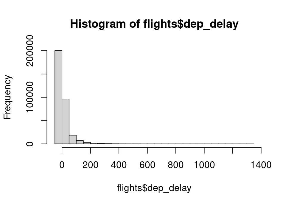
boxplot(flights$dep_delay)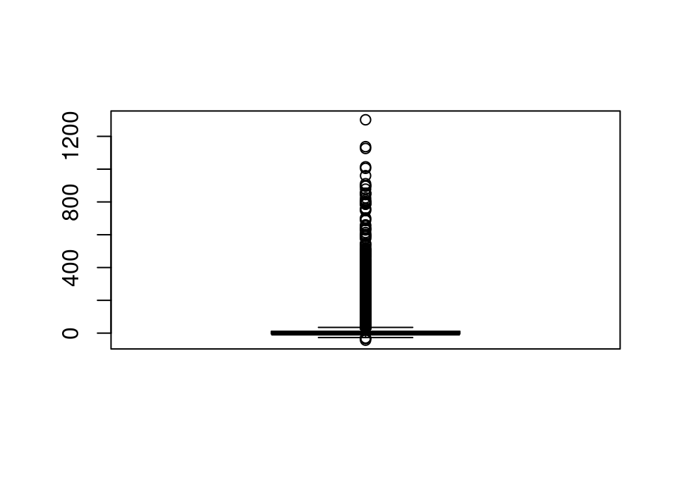
hist(flights |> filter(dep_delay <= 120) |> pull(dep_delay))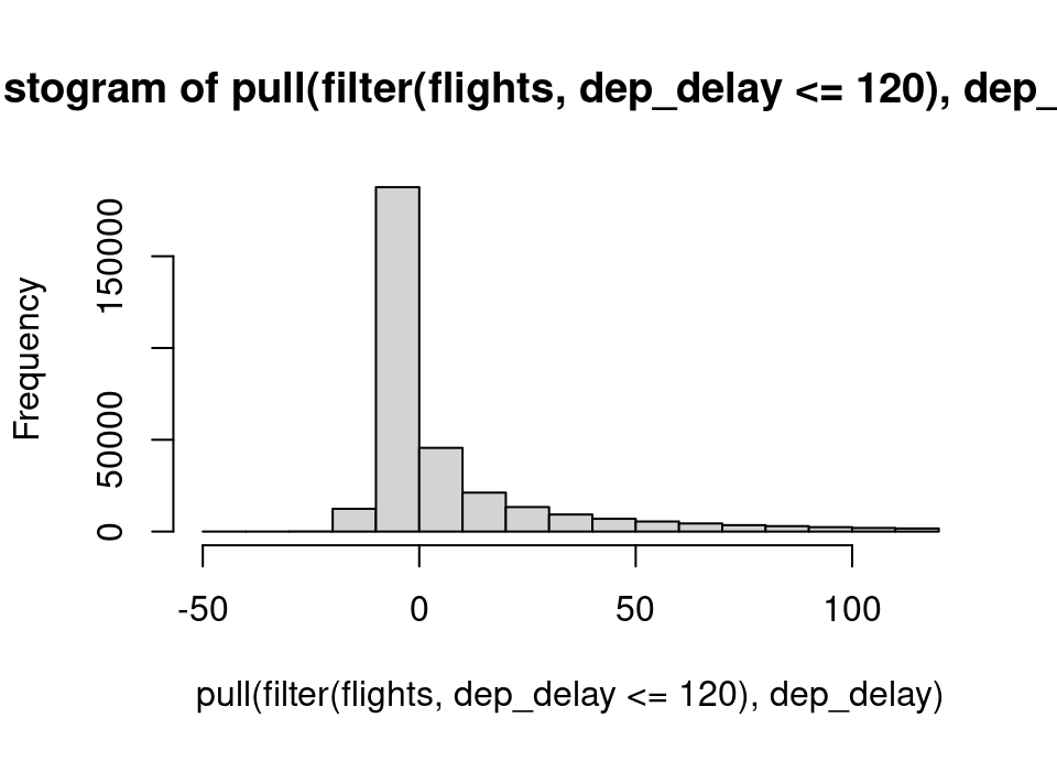
boxplot(flights |> filter(dep_delay <= 120) |> pull(dep_delay))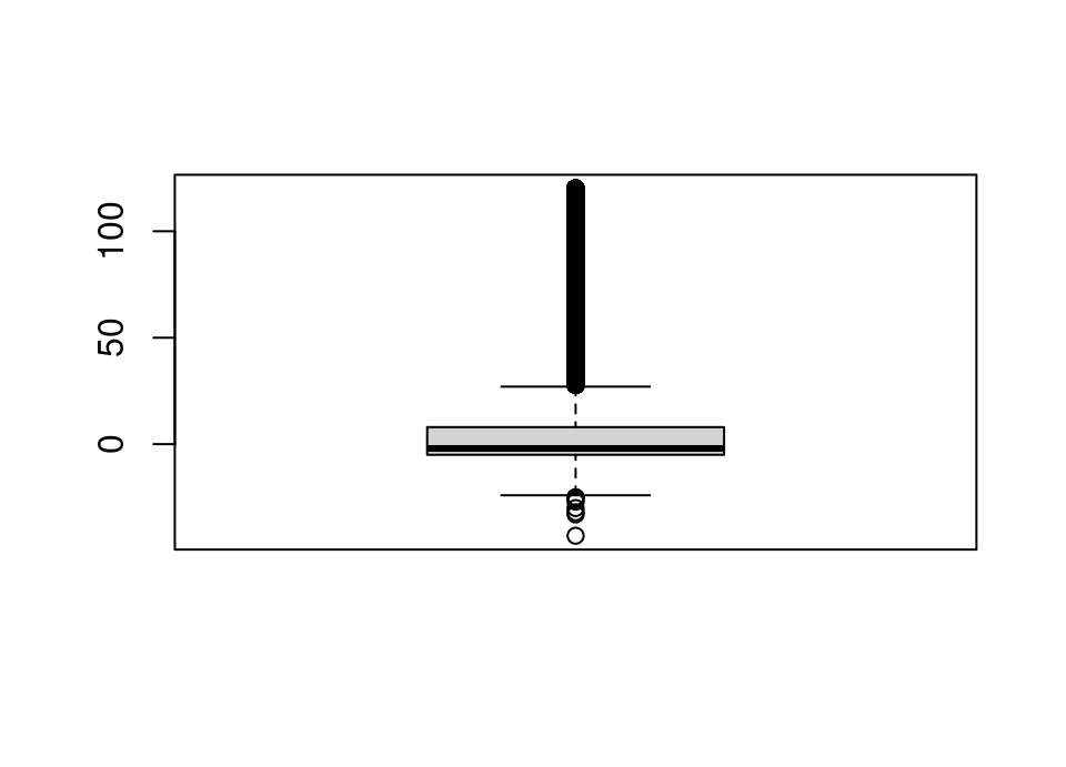
For the following exercise you’ll need a new function you’ve not seen before, called ifelse().
It takes exactly 3 arguments.
- The first should be a vector of logical conditions
- The second should be any vector of the same length as the first argument
- The third should also be any vector of the same length as the first argument
It works by returning a new vector which contains the corresponding elements of the second vector wherever there is a TRUE in the first vector, and the corresponding elements of the third vector wherever there is a FALSE in the second vector.
For example:
ifelse(c(TRUE, TRUE, FALSE, TRUE, FALSE),
       c(1, 2, 3, 4, 5),
       c(1000, 2000, 3000, 4000, 5000))
[1] 1 2 3000 4 5000This allows you to use the function to selectively do different things. For example, I could sample some random numbers and then replace all values over a certain size with a threshold value:
x <- rexp(10)
x
[1] 1.3150899 0.6896679 0.5015532 1.8022444 4.9024758 0.2578629 0.1227773
[8] 0.8719619 1.8942236 1.4993733x <- ifelse(x > 1,
rep(1, 10),
x)
x [1] 1.0000000 0.6896679 0.5015532 1.0000000 1.0000000 0.2578629 0.1227773
[8] 0.8719619 1.0000000 1.0000000Exercise 5.61 Counting leaving early as negative is cheating! It might skew our impression of the average delay when a delay does occur.
Recompute the average, standard deviation and count of departure delay when you change any early departure to be a delay of 0 instead of a negative time.
Does your conclusion change?
Click for solution
## SOLUTION

flights |>
  mutate(dep_delay = ifelse(dep_delay < 0, 0, dep_delay)) |>
  group_by(carrier) |>
  summarise(avg_dep_delay = mean(dep_delay, na.rm = TRUE),
            sd_dep_delay = sd(dep_delay, na.rm = TRUE),
            num_flights = n())
# A tibble: 16 × 4
carrier avg_dep_delay sd_dep_delay num_flights
<chr> <dbl> <dbl> <int>
1 9E 19.8 44.4 18460
2 AA 11.8 36.2 32729
3 AS 9.95 29.7 714
4 B6 15.8 37.2 54635
5 DL 11.9 38.8 48110
6 EV 22.7 45.1 54173
7 F9 22.6 57.3 685
8 FL 21.2 51.5 3260
9 HA 9.05 73.5 342
10 MQ 14.3 37.6 26397
11 OO 18 40.4 32
12 UA 14.1 34.8 58665
13 US 7.94 26.6 20536
14 VX 14.9 44.0 5162
15 WN 18.9 42.8 12275
16 YV 22.6 47.3 601Exercise 5.62 The times given in the variables ending _time are clock times, which are nice and easy to interpret, but we can’t calculate easily with them (1300 is one minute later than 1259, not 41 minutes later!)
Create a new function called clock_to_minutes which takes a clock time like 1259 and converts it to the number of minutes since midnight (for example, \(1259 \to 779\))
Hint: one of the functions floor, ceiling or round might assist, look at their help file to choose which to use.
Click for solution
## SOLUTION

clock_to_minutes <- function(time) {
  floor(time/100)*60 + (time-floor(time/100)*100)
}

# Check we get expected result on the example in the Q
clock_to_minutes(1259)
[1] 779Exercise 5.63 Use your function to modify the dep_time and arr_time columns to record minutes since midnight, instead of clock time.
Click for solution
## SOLUTION

flights2 <- flights |>
  mutate(dep_time = clock_to_minutes(dep_time),
         arr_time = clock_to_minutes(arr_time))

head(flights2)
# A tibble: 6 × 19
year month day dep_time sched_dep_time dep_delay arr_time sched_arr_time
<int> <int> <int> <dbl> <int> <dbl> <dbl> <int>
1 2013 1 1 317 515 2 510 819
2 2013 1 1 333 529 4 530 830
3 2013 1 1 342 540 2 563 850
4 2013 1 1 344 545 -1 604 1022
5 2013 1 1 354 600 -6 492 837
6 2013 1 1 354 558 -4 460 728
# ℹ 11 more variables: arr_delay <dbl>, carrier <chr>, flight <int>,
# tailnum <chr>, origin <chr>, dest <chr>, air_time <dbl>, distance <dbl>,
# hour <dbl>, minute <dbl>, time_hour <dttm>Exercise 5.64 Finally, you may have noticed when working with this data that there are quite a few NA values.
These represent scheduled flights that were cancelled.
How many flights were cancelled in total?
Create a table showing the total number of cancellations by the hour of scheduled departure, sorted in descending order by the count.
That last table might be misleading given that there are very different numbers of flights at different times of day. Repeat the analysis, but calculating the proportion of flights cancelled each hour of the day. Would you choose to fly before or after lunch?
Click for solution
If you look at the data, you’ll see the NAs occur in departure and arrival time columns, among others (those that record actual flight information, rather than scheduled information).
## SOLUTION

# Total flights cancelled
flights |>
  filter(is.na(dep_time)) |>
  nrow()
[1] 8255# Flights cancelled by hour of day
flights |>
filter(is.na(dep_time)) |>
mutate(sched_dep_time = floor(sched_dep_time/100)) |>
group_by(sched_dep_time) |>
summarise(cancelled = n()) |>
arrange(desc(cancelled))# A tibble: 20 × 2
sched_dep_time cancelled
<dbl> <int>
1 19 861
2 16 840
3 15 670
4 17 660
5 20 636
6 18 626
7 14 566
8 8 442
9 13 429
10 6 425
11 21 409
12 12 388
13 9 327
14 11 296
15 10 290
16 7 289
17 22 78
18 23 13
19 5 9
20 1 1# Proportion cancelled by hour of day
flights |>
mutate(sched_dep_time = floor(sched_dep_time/100)) |>
group_by(sched_dep_time) |>
summarise(total = n(), cancelled = sum(is.na(dep_time))) |>
mutate(prop = cancelled/total) |>
arrange(desc(prop))# A tibble: 20 × 4
sched_dep_time total cancelled prop
<dbl> <int> <int> <dbl>
1 1 1 1 1
2 19 21441 861 0.0402
3 20 16739 636 0.0380
4 21 10933 409 0.0374
5 16 23002 840 0.0365
6 22 2639 78 0.0296
7 18 21783 626 0.0287
8 15 23888 670 0.0280
9 17 24426 660 0.0270
10 14 21706 566 0.0261
11 13 19956 429 0.0215
12 12 18181 388 0.0213
13 11 16033 296 0.0185
14 10 16708 290 0.0174
15 6 25951 425 0.0164
16 8 27242 442 0.0162
17 9 20312 327 0.0161
18 7 22821 289 0.0127
19 23 1061 13 0.0123
20 5 1953 9 0.00461🏁🏁 Done, end of lab! 🏁🏁