Assignment 3 Solutions
Q1
The following integral is difficult to evaluate analytically: \[ \int_{-1}^1 \frac{x^2}{\sqrt{x^2+4}} \,dx \]
Express the integral as an expectation with respect to a Uniform distribution and write down the Monte Carlo estimator of this integral given simulations \(\{ x_1, \dots, x_n \}\) from a Uniform\((-1,1)\).
\[\begin{align*} \int_{-1}^1 \frac{x^2}{\sqrt{x^2+4}} \,dx &= \int_{-1}^1 \left( \frac{2x^2}{\sqrt{x^2+4}} \right) \underbrace{\frac{1}{2}}_{\text{Uniform(-1,1) pdf}} \,dx \\ &= \mathbb{E}_X\left[ \frac{2X^2}{\sqrt{X^2+4}} \right] \quad \text{for }X\text{ Uniform(-1,1)} \end{align*}\]
\[\hat{\mu}_n = \frac{1}{n} \sum_{i=1}^n \frac{2x_i^2}{\sqrt{x_i^2+4}}\]
Q2
The function \(f_X(x) = \frac{3}{2} x^2\) is a valid probability density function for a random variable \(X \in [-1,1]\), and \(X\) can easily be simulated (we will see how soon!)
Express the integral as an expectation with respect to the random variable \(X\) having this pdf, and write down the Monte Carlo estimator of this integral given simulations \(\{ x_1, \dots, x_n \}\) of \(X\).
\[\begin{align*} \int_{-1}^1 \frac{x^2}{\sqrt{x^2+4}} \,dx &= \int_{-1}^1 \left( \frac{2}{3\sqrt{x^2+4}} \right) \underbrace{\frac{3}{2}x^2}_{\text{pdf }f(x)} \,dx \\ &= \mathbb{E}_X\left[ \frac{2}{3\sqrt{X^2+4}} \right] \quad \text{for }X\text{ following }f(x) \end{align*}\]
\[\hat{\mu}_n = \frac{1}{n} \sum_{i=1}^n \frac{2}{3\sqrt{x_i^2+4}}\]
Q3
You do a pilot simulation and find the terms in the Monte Carlo estimator for (Q1) have variance \(0.0731\), whilst for (Q2) they have variance \(8.12 \times 10^{-5}\). Determine how many simulations would be needed to achieve a RMSE of \(0.00005\) in each case.
The RMSE is:
\[\frac{\sqrt{\text{Var}(Y)}}{\sqrt{n}}\]
We can use the simulations to also estimate \(\text{Var}(Y)\) in each case. Therefore, for the Uniform case, we need:
\[\begin{align*} \frac{\sqrt{\text{Var}(Y)}}{\sqrt{n}} &= 0.00005 \\ \implies n &= \frac{0.0731}{0.00005^2} \\ &= 29,240,000 \end{align*}\]
That is, we need \(29,240,000\) simulations where \[Y = \frac{2X^2}{\sqrt{X^2+4}}\]
For \(f(x)\), we need:
\[\begin{align*} \frac{\sqrt{\text{Var}(Y)}}{\sqrt{n}} &= 0.00005 \\ \implies n &= \frac{8.12 \times 10^{-5}}{0.00005^2} \\ &= 32,480 \end{align*}\]
Thus, we need \(32,480\) simulations where \[Y = \frac{2}{3\sqrt{X^2+4}}\]
Q4

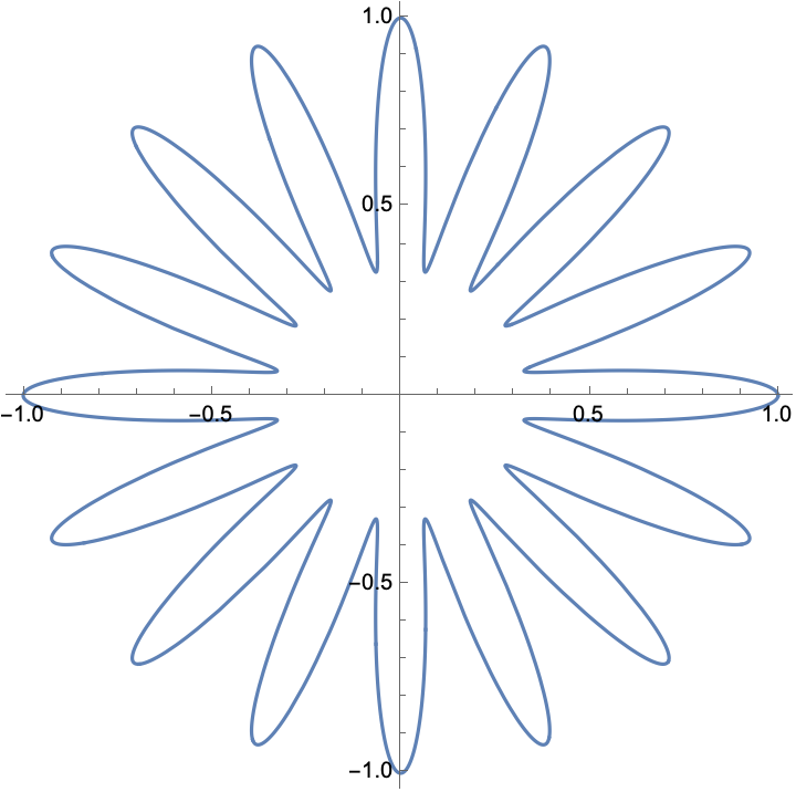
The area inside the blue curved “flower” above is defined in polar coordinates as the region,
\[\left\{ (r, \theta) : r \le \frac{2}{3} + \frac{1}{3} \cos(16 \theta), \ 0 \le \theta \le 2\pi \right\}\]
Note: you do not need to do lots of algebra here, think about this particular problem geometrically.
Write R code to estimate the area within the flower based on Uniform simulations on the square \([-1,1]^2\) (just like we estimated \(\pi\) in lectures). Run this code to create a Monte Carlo estimate based on \(10,000\) simulations from the square and provide a 95% confidence interval for your estimate.
Hint: you may find the R function
atan2()useful, see “Details” on the function help page.
n <- 10000
x <- runif(n, -1, 1)
y <- runif(n, -1, 1)

p.hat <- mean(sqrt(x^2+y^2) <= 2/3 + 1/3*cos(16*atan2(y,x)))
p.std.err <- sqrt((p.hat*(1-p.hat))/n)

A.hat <- 4*p.hat
A.ci <- 4*(p.hat + c(-1,1)*1.96*p.std.err)

A.hat
[1] 1.5548A.ci[1] 1.516584 1.593016It was not asked in the question, but notice the size of the CI here is 0.0764329.
Q5
Notice that the flower is contained entirely within the circle of radius 1 centred at \((0,0)\). It is probably more natural given the polar form to produce your Monte Carlo estimate using uniform simulations in the circle.
Write R code which simulates a uniformly random point in the circle by simulating \(\theta \sim \text{Unif}(0, 2\pi)\) and \(r^2 \sim \text{Unif}(0,1)\), then use this code to create a Monte Carlo estimate based on \(10,000\) simulations from the circle and provide a 95% confidence interval for your estimate.
Hint: simulate a Uniform on \((0,1)\) and take the square root to simulate \(r\) above.
Aside: it may initially seem counter-intuitive, but if you simulate \(r\) as just a straight Uniform, then you do not end up with points uniformly distributed over the circle because the density of points near the origin will be too high. The square root transformation ensures uniformity over the circle.
n <- 10000
theta <- runif(n, 0, 2*pi)
r <- sqrt(runif(n, 0, 1))

p.hat <- mean(r <= 2/3 + 1/3*cos(16*theta))
p.std.err <- sqrt((p.hat*(1-p.hat))/n)

A.hat <- pi*p.hat
A.ci <- pi*(p.hat + c(-1,1)*1.96*p.std.err)

A.hat
[1] 1.582106A.ci[1] 1.551319 1.612893It was not asked in the question, but notice that the size of the CI here is 0.0615736, which should be smaller than in Q4 for the same simulation size \(n\).
🏁🏁 Done, end of assignment! 🏁🏁