Lab 2: Scripts, Loops, and MC Testing
🧑💻 Make sure to finish Lab 1 before continuing with this lab! I have brought forward the “extra” material that was on Monte Carlo hypothesis testing which some of you may not have got to do last week due to the lecturing timing: it appears after the initial sections on using script files in RStudio and warm-up looping exercises.
NOTE: if you are using the Github Codespace and get a popup error saying something about a previous session crashing, this just means you didn’t follow the instructions on the the appendix page “R and RStudio” linked here properly when ending the last session … you should always press the red standby button at the very top right of the page, then use the bottom left button to stop the codespace before closing the browser! Don’t worry, nothing bad has happened, but you can avoid the error in future by shutting down everything cleanly – don’t hesitate to ask if you’re unsure.
Script files 📜
Last week we wanted to get going quickly, so you just used RStudio in interactive mode. However, it is usually better to write code in a script file and then run that code. Create a new script file as follows …


There are several advantages to using script files, including:
You can now type in the new script panel like a regular text document. When you press Enter it will not run code, but will allow you to write multiple lines, and you can easily go back and edit text etc. All the code completion help and tool tips which we discussed in the lecture will still be provided by RStudio.
Once you are happy the code is how you want it to run, simply place the cursor anywhere on the line you want to run and press the key combination
Cmd+Enter(Mac) orCtrl+Enter(Windows/Linux). That will trigger RStudio to automatically copy the command down to the Console and run it. Note:- The cursor automatically moves to the next line of code, so you can run multiple lines in quick succession by keeping
Cmd(Mac) orCtrl(Windows/Linux) pressed and tappingEnterrepeatedly. - If you do this on the first line of a block of code (like a for loop) then the whole loop is copied and run automatically.
- If you want to run a whole bunch of code without tapping repeatedly as mentioned above, you can instead highlight the exact code you want to run before pressing the key combination
Cmd+Enter(Mac) orCtrl+Enter(Windows/Linux). As well as allowing you to run multiple lines at one, you can also highlight just part of a single line to run.
Try this now and be sure it works before carrying on … this is important and useful, so if it is not working be sure to ask for help 🙋♀️
- The cursor automatically moves to the next line of code, so you can run multiple lines in quick succession by keeping
You can now save your code between sessions. Note that if you’re using the Github Codespace, then your code is saved on the server and not the machine you’re accessing it from. If you want to download the code this is easily done by ticking next to the file you want in the Files pane, then click the cog (in the Files pane) and choose “Export …”.
You can have many script files open at once. We’re probably not going to need that in the labs, but when working on large scale real-life projects, it is common to divide up the project logically into different files (eg files for loading data; other files for transformation, manipulation and cleaning that data; other files for building statistical and machine learning models; yet other files for deployment of those models into production settings etc)
Ok … on to the coding part of the lab! Be sure to use a script file and the hints above when writing your code from now on. At the end of the lab, save the file for future learning/reference.
Simple looping calculations
Now that we have looked at loops and vectors in the practical lecture, we’ll do a warm-up exercise which isn’t Statistics at all, doing some simple computations with factorials.
The factorial is defined to be: \[n! := \prod_{k=1}^n k\]
Exercise 5.8 We can write a for loop to compute the factorial. Copy the code below and replace the ??? to correctly compute \(100!\)
x <- 1
for(k in ???) {
  x <- x*???
}
print(x)
Click for solution
## SOLUTION
x <- 1
for(k in 2:100) {
  x <- x*k
}
print(x)
[1] 9.332622e+157One of the nice things about R is that vector can be used nearly everywhere. So using a for loop is rather inefficient for the above. Instead we can use a built in function and just supply a vector of values.
Exercise 5.9 To be more efficient, create a vector containing all the integers from 1 to 100 inclusive and use the prod() function to find the factorial.
Click for solution
## SOLUTION
prod(1:100)
[1] 9.332622e+157Of course, all the above is unnecessary because there is a built-in function to compute the factorial for us.
Exercise 5.10 Compute \(100!\) factorial using the built-in function factorial() and confirm it agrees with your manual calculations above.
Click for solution
## SOLUTION
factorial(100)
[1] 9.332622e+157Stirling’s approximation provides an asymptotic formula for calculating the factorial: \[n! \approx \left(\frac{n}{e}\right)^n \sqrt{2 \pi n}\]
Exercise 5.11 Create two vectors of length 100, one named exact and one named stirling, and then by writing a for loop (or otherwise) fill the \(k\)th element with \(k!\) computed either exactly or using the Stirling approximation respectively.
(ie exact[23] should contain \(23!\) and stirling[23] should contain \(\left(\frac{23}{e}\right)^{23} \sqrt{2 \pi \times 23}\) etc)
Click for solution
## SOLUTION
exact <- rep(1, 100)
stirling <- rep((1/exp(1)) * sqrt(2*pi), 100)
for(k in 2:100) {
  exact[k] <- k*exact[k-1]
  stirling[k] <- (k/exp(1))^k * sqrt(2*pi*k)
}
Recall that the relative error between a true value \(x\) and an approximation \(\hat{x}\) is defined to be \[\left|\frac{\hat{x} - x}{x}\right|\]
Also recall from the lecture that we can perform element-wise operations on vectors very easily!
Exercise 5.12 By using element-wise operations on the exact and stirling vectors you created above, compute the relative error and store it in a variable called rel.err by replacing the ??? below.
The two commands after it create simple scatter plots of the relative error in computing \(k!\) using Stirling against the value \(k\). The second is on the \(\log_{10}\) scale which is easier to interpret since we can immediately deduce the number of leading zeros in the relative error.
rel.err <- ???
plot(1:length(rel.err), rel.err, xlab = "k")
plot(1:length(rel.err), log10(rel.err), xlab = "k")
Click for solution
## SOLUTION
rel.err <- abs((stirling-exact)/exact)
plot(1:length(rel.err), rel.err, xlab = "k")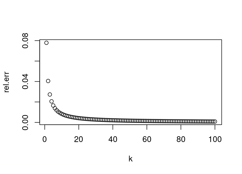
plot(1:length(rel.err), log10(rel.err), xlab = "k")
With those toy warm-up exercises out of the way, let’s now turn to some problems based on the lecture material we’re covering.
Monte Carlo hypothesis testing
We saw in lectures that we can avoid having to compute the sampling distribution of the test statistic for a hypothesis test by instead just simulating a lot of ‘fake’ or pseudo datasets from the null distribution and then seeing whether the observed test statistic is extreme by comparison.
In the lecture practical, we saw that we can simulate throwing a dice 60 times with the following code:
table(sample(1:6, 60, replace = TRUE))
 1  2  3  4  5  6
 6 11 11 13 12  7
Exercise 5.13 By looking at the help file for sample, find out how to make the dice biased, so that 6 comes up with probability 0.25 and each other face with probability 0.15.
Roll this dice 60 times.
Click for solution
## SOLUTION
table(sample(1:6, 60, replace = TRUE, prob = c(0.15, 0.15, 0.15, 0.15, 0.15, 0.25)))
 1  2  3  4  5  6
 5 12 11  6  7 19
Now that we have our biased dice, can you think of a test statistic which would be ‘extreme’ when the dice is biased and ‘not extreme’ when the dice is fair? Note: feel free to be creative … don’t worry at the moment what the optimal choice might be! The idea is that you get comfortable with the core concept of hypothesis testing and why simulation can be used to do it.
Exercise 5.14 Perform a Monte Carlo hypothesis test of whether the dice above is fair.
Replace the first ??? with your biased dice roll code and replace the second and third ??? with your proposed test statistic.
x <- ???

obs.test.stat <- ???

test.stat <- rep(0, 10000)
for(i in 1:10000) {
  sim <- table(sample(1:6, 60, replace = TRUE))

  test.stat[i] <- ???
}
mean(test.stat > obs.test.stat)
Click for solution
## SOLUTION
x <- table(sample(1:6, 60, replace = TRUE, prob = c(0.15, 0.15, 0.15, 0.15, 0.15, 0.25)))

obs.test.stat <- sum((x-10)^2)

test.stat <- rep(0, 10000)
for(i in 1:10000) {
  sim <- table(sample(1:6, 60, replace = TRUE))

  test.stat[i] <- sum((sim-10)^2)
}
mean(test.stat > obs.test.stat)
[1] 0.8381Explore how the above behaves as you try making the dice more and more biased. Also, try different ideas for test statistic – can you see which might be performing better?
Exploring MC testing
We’re interested in empirically exploring the behaviour of Monte Carlo testing. This complements the Tutorial this week, where you will look at some of these aspects theoretically.
- Is Monte Carlo testing always right, in the sense of agreeing with the theoretically exact conclusion?
- How does the Monte Carlo estimator convergence behave?
- If I have more than one idea for a test statistic, are they necessarily equally good choices?
We will look at just the first of these, but may return to the other questions another time … have a think about them in the mean time!
When analysing the behaviour of a method, it is convenient to consider a problem where we can calculate the theoretical answer exactly so that we can compare how Monte Carlo testing is doing (of course, in reality we usually resort to Monte Carlo testing in the cases where we don’t know the exact solution). Let’s use the World War II tanks example from the lecture, since it has a particularly easy form for the exact answer! 🪖
Exercise 5.15 Use R to calculate the exact p-value, if we now perform the one-sided test that the German army might have \(N=107\) tanks versus fewer (ie a different null value to the lecture, otherwise all the same).
If the significance level of your test was \(\alpha=0.05\), would you reject or not reject the null hypothesis.
Click for solution
We can calculate this by manually typing everything in:
## SOLUTION

61/107 * 60/106 * 59/105 * 58/104 * 57/103
[1] 0.05596113Or, if you’re using the methods we learned in lectures, you could abbreviate this to:
## SOLUTION

prod((61:57)/(107:103))
[1] 0.05596113Exercise 5.16 Write code which will perform a Monte Carlo version of the above hypothesis test.
Remember, this involves simulating from the null distribution: what is that here? How do we do so in R?
Use a variable M to store the number of Monte Carlo simulations your code uses, so that you can easily change the value of M and rerun for a different number of iterations.
To begin with use M <- 1000 iterations.
Once you have your code working, run it several times and look at how the p-value varies … each time think about whether you would reject or not at \(\alpha=0.05\).
Click for solution
The null distribution is just Uniform sampling without replacement on \(\{1,\dots,107\}\). We can achieve this with the sample function, being careful about with/without replacement sampling.
We’ll use M to denote the number of Monte Carlo iterations to avoid confusion with \(N\) being the total number of tanks.
## SOLUTION

# Tank data and null
x <- c(61, 19, 56, 24, 16)
N0 <- 107

# Simulate M sets of data of size 5, assuming the null is true
M <- 1000
t <- rep(0, M)
for(j in 1:M) {
  # Sampling is from the set of values {1,...,N0} without replacement
  z <- sample(1:N0, 5)
  t[j] <- max(z)
}

# Calculate empirical p-value
sum(t <= max(x)) / M
[1] 0.046If you rerun this code many times with M <- 1000, you should get the p-value jumping around quite a lot and in particular sometimes crossing the “wrong” side of \(\alpha=0.05\) compared to the theoretically exact answer.
Exercise 5.17 Take your solution to the last exercise and by wrapping it all in an outer for loop, create a new vector called pvals in which you store 1000 simulations of the p-value.
In other words, your outermost loop is going to do 1000 experiments. Each experiment is itself a loop doing 1000 Monte Carlo simulations in order to find a p-value. Hence, you end up with 1000 p-values (each found using 1000 simulations of the null).
Hint: be very careful to use a different variable name in each for loop so that they don’t conflict!
NOTE: this might take 5-10 seconds to run.
Click for solution
## SOLUTION

# Tank data and null
x <- c(61, 19, 56, 24, 16)
N0 <- 107

# Wrap the important code from earlier in an outer for loop and
# fill up the pvals vector
pvals <- rep(0, 1000)
for(i in 1:1000) {
  # Simulate M sets of data of size 5, assuming the null is true
  M <- 1000
  t <- rep(0, M)
  for(j in 1:M) {
    # Sampling is from the set of values {1,...,N0} without replacement
    z <- sample(1:N0, 5)
    t[j] <- max(z)
  }
  # Calculate empirical p-value
  pvals[i] <- sum(t <= max(x)) / M
}
Once you have created the vector pvals, copy/paste and run the following code (we haven’t done graphics yet, so don’t worry about understanding this in detail yet … coming to a lecture soon! For now, focus on interpreting the output)
library("MASS")
truehist(pvals, xlim = c(0.03, 0.08))
abline(v = 0.05, col = "red", lwd = 4)
abline(v = 0.05596113, col = "purple", lwd = 4)
This creates a histogram showing how spread out the Monte Carlo simulated p-values are, with a red line showing the significance level \(\alpha=0.05\) and a purple line showing the theoretically exact p-value. It should look like the following (click to see in solution):
Click for solution
We can see here that the p-values are at least centred on the true value (the purple line), but what might be worrying is that a large part of the left tail is below the red line … in other words, on the opposite side of the \(\alpha=0.05\) significance level.
Attaching package: 'MASS'The following object is masked from 'package:dplyr':
select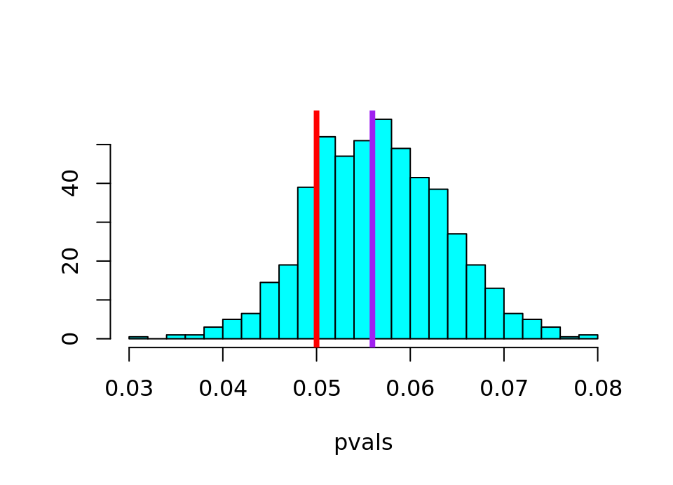
Exercise 5.18 What percentage of the 1000 Monte Carlo p-values reached the wrong conclusion at a significance level \(\alpha=0.05\)?
Click for solution
The Monte Carlo test would lead to the wrong conclusion if the estimated p-value is the opposite side of the significance level from the theoretically exact p-value … in other words, any Monte Carlo p-values less than 0.05 would lead us to the wrong test conclusion.
## SOLUTION

100 * sum(pvals<0.05)/1000
[1] 17.9Exercise 5.19 Repeat all the above steps, with M <- 2000 instead (will take twice as long to run). What do you notice?
Click for solution
## SOLUTION

# Tank data and null
x <- c(61, 19, 56, 24, 16)
N0 <- 107

# Wrap the important code from earlier in an outer for loop and
# full up the pvals vector
pvals <- rep(0, 1000)
for(i in 1:1000) {
  # Simulate M sets of data of size 5, assuming the null is true
  M <- 2000
  t <- rep(0, M)
  for(j in 1:M) {
    # Sampling is from the set of values {1,...,N0} without replacement
    z <- sample(1:N0, 5)
    t[j] <- max(z)
  }
  # Calculate empirical p-value
  pvals[i] <- sum(t <= max(x)) / M
}

library("MASS")
truehist(pvals, xlim = c(0.03, 0.08))
abline(v = 0.05, col = "red", lwd = 4)
abline(v = 0.05596113, col = "purple", lwd = 4)
100 * sum(pvals<0.05)/1000[1] 11.2🏁🏁 Done, end of lab! 🏁🏁