Lab 1: Introduction to R
Due to the impossibility of University central timetabling to ensure the lectures happen before any of the practicals, some people will have a practical before the first lecture! This lab is therefore a gentle introduction to make sure you can access R, try out some simple code and then revise some first-year statistics concepts that will be useful. The more fun statistics and data science will come to a practical near you in the future!
The idea is that in these labs you have time to work through a lab sheet like this, with someone experienced on hand to answer any questions you may have. Don’t hesitate to put your hand up to ask a question! 🙋♀️ Whoever is taking the lab (it might be your lecturer Dr Louis Aslett, or either Prof Jochen Einbeck or Adam Iqbal) will come to you as soon as possible.
Finally, this being the first lab, there’s a lot of extra explanatory text to guide you through how to get going and use these labs, but please do bear with the amount to read and go through it all. This style is intentionally informal to try to make it easier to read … although you could rush through and probably finish well before the 50 minute lab ends, it is better to cover everything carefully!
Software setup
We will use the Integrated Development Environment (IDE) called RStudio on this course, because it is arguably the most powerful of the environments to develop R code in, and is used extensively in research and industry.
There are 3 options for how to run RStudio for these labs, with running on a Github Codespaces image that I have prepared being the recommended option. Please visit the appendix page “R and RStudio” linked here and first make sure that you can start RStudio using one of the 3 options provided, then come back to this page to carry on with the lab.
Getting started
For this first simple lab, we will just use R in “interactive mode”, where you type in code and immediately execute it by hitting enter. To do this, simply click at the console prompt indicated in the following image and type there.
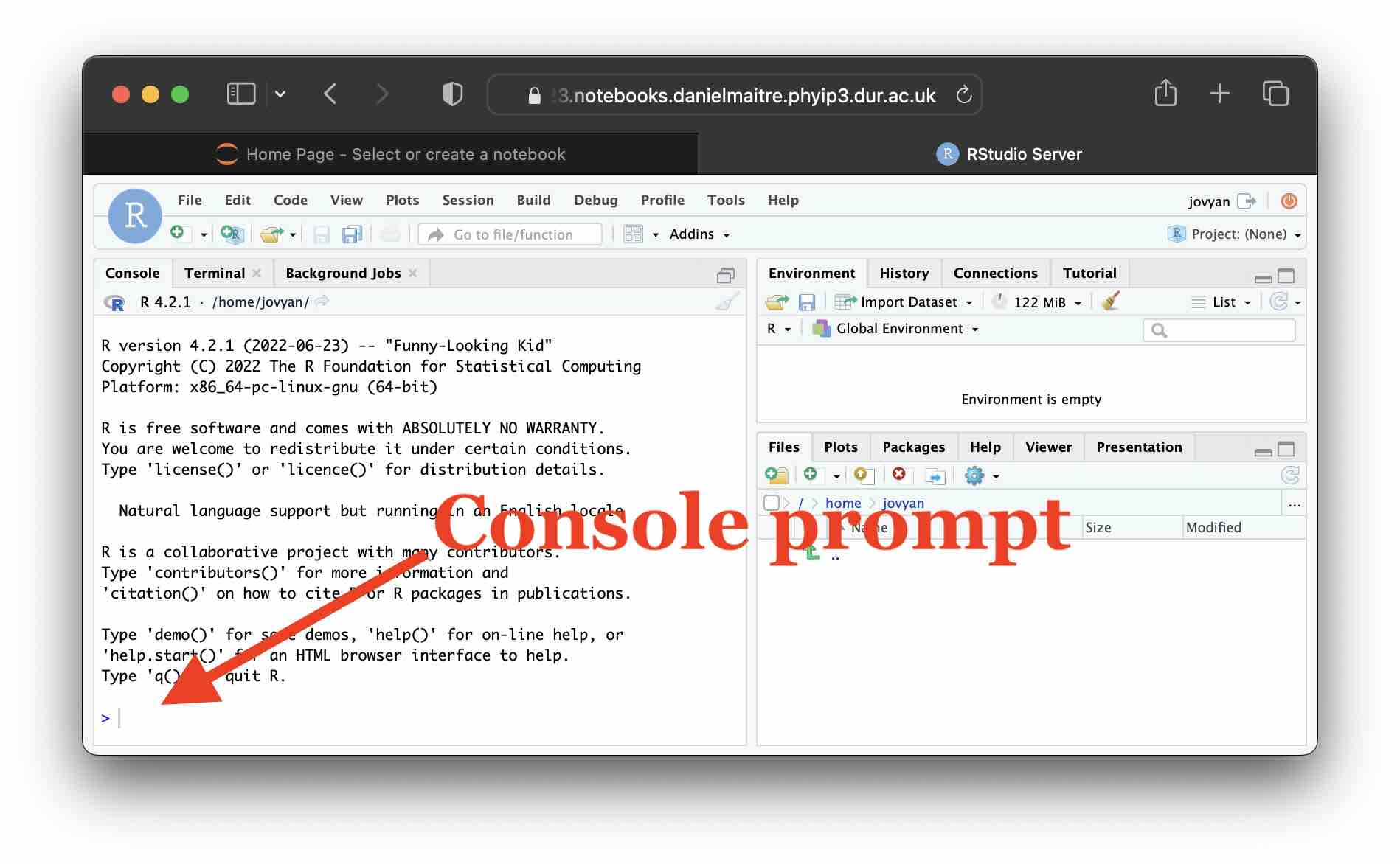
RStudio is very powerful and has many time saving features, so we will discuss the other parts of the RStudio interface as the lectures progress.
A simple calculator! 🧮
We could just treat R like a calculator and type in arithmetic expressions to have R evaluate the result. For example, try:
2+3and after hitting enter you should see:
[1] 5You can ignore the [1] prefix, the result obviously being 5 … we will see in lectures what the prefix means.
Each row of the following table has a very basic examples of a mathematical expression in the left hand column, and how to code them in R in the right hand column.
| \(\sqrt{2}\) | sqrt(2) |
| \(2 \times 3\) | 2*3 |
| \(2^3\) | 2^3 |
| \(2 \div 3\) | 2/3 |
| \(\log_{10}{2}\) | log10(2) |
| \(\pi\) | pi |
| \(\log_e{2}\) | log(2) |
| \(\sin{2}\) (in radians) | sin(2) |
| \(e\) | exp(1) |
| \(e^2\) | exp(2) |
| \(5 \bmod{2}\) | 5%%2 |
Play around with running some of these until you’re happy with how it works.
Next, we’ll have a first Exercise. Every exercise in these labs has a solution which can be revealed by clicking within the dashed box immediately below it. However,
- I would strongly urge you to really try hard to come up with a solution before you click to reveal it … the labs are not a race and we tend to remember solutions to things better if we’ve wrangled a bit with them first;
- Do look at the solution even if you have solved the exercise yourself … sometimes the solution includes some extra discussion about interesting or important learning points from the exercise.
Exercise 5.1
Using R, confirm that \(e^\pi > \pi^e\) by evaluating each side of the inequality.Click for solution
This apparently simple exercise already highlights an important point which is implicit in the table above!
We access \(e\) always via a function which evaluates \(e^x\) for some \(x\), whilst \(\pi\) is provided as a constant.
That leads to possibly surprising looking code for calculating \(\pi^e\).
## SOLUTION

exp(pi)
[1] 23.14069pi^exp(1)[1] 22.45916Note that if you were in a contrary mood then of course you might have used the table of expressions above very literally and therefore may have typed exp(1)^pi for \(e^\pi\) … this would work but is rather suboptimal!
🧐 So clearly we must think carefully about what kind of ‘thing’ (eg a function, a constant, etc) the object we’re working with is.
If we’d mistakenly treated pi as a function and written pi(exp(1)) would the error message have helped?
Try it … type in the incorrect code!
exp as a constant): would the error message when you type exp^pi help you?
Some error messages are more helpful/easier to interpret than others, so you’ll need to develop your detective skills in interpreting R error messages!
🕵️ Also, notice that R doesn’t bite, so don’t be afraid to just experiment sometimes.
Of course, this is of pretty limited interest.
At the very least, we will want to be able to assign our results to a variable.
If I wish to store \(\sqrt{2}\) in a variable x, then the idiomatic R syntax for this is:
x <- sqrt(2)where the <- is formed by typing < followed by - (the font on this page may make the two characters look joined).
Note that while it is possible to use = instead of <- (and most of the time it will behave as expected), it is not recommended.
In a future lecture when we have covered more details I will elaborate on why it is preferable to avoid = for assigning to a variable … so try to adopt the habit of using <- from the start!
If you type the above command into R and hit enter, you will immediately get the prompt back and it may seem that nothing has happened!
Fear not, when you assign to a variable this suppresses outputting the value, but if you now type x and hit enter you can examine the result:
x[1] 1.414214You can also further manipulate x, so for example x^2 would return 2 and cos(pi/4)*x would return 1, as expected.
Functions
We have been using and referred to functions above. In a nut shell, a function is an encapsulation of some other code. We can call that code and provide arguments to it, and it will return some result which we either use as part of an expression, store in a variable, or inspect directly.
For example, when I typed cos(pi/4) above:
- the function is
cos - the function takes a single argument, which here was
pi/4 - the whole of that code is evaluated and will return \(\frac{1}{\sqrt{2}}\) which we can just have print out to the console, store or directly use in an expression like above, where I wrote
cos(pi/4)*x
Functions are much more flexible than demonstrated by cos and may take more than a single argument.
Click on the “Help” tab in the bottom right panel as highlighted here:
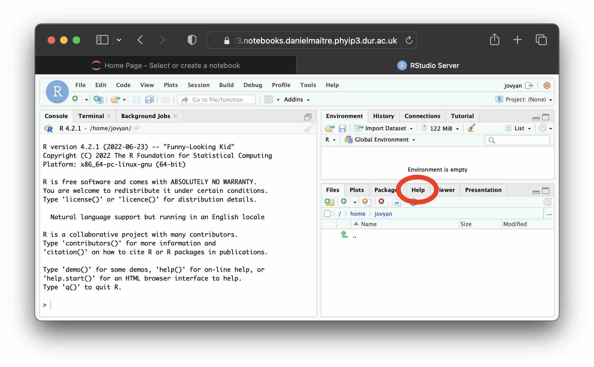 and in the search bar revealed immediately below, search for
 log and hit enter.
This brings up a help page all about that function, and you can use it to search on any other object in R.
Skim read the first few sections of the documentation page for log.
You should have noticed when you got to the “Usage” section, the definition reads log(x, base = exp(1)), which indicates that log can take more than one argument.
In particular,
- The first argument is named
xand we must provide it; - The second argument is named
base, but the= exp(1)indicates that it has a default value … in other words, if we don’t supply the second argument then it is assumed to be \(e\).
Exercise 5.2
Compute \(\log_{10} \pi\) using both thelog10 and log functions.
Click for solution
## SOLUTION

log10(pi)
[1] 0.4971499log(pi, 10)[1] 0.4971499An important and very useful final fact about function arguments is that R allows you to refer to them by name, so log(pi, base = 10) also gives the same result.
In fact, once you name arguments R will allow you to give the named ones in any order and then matches the unnamed ones in the order they appear to any remaining unspecified arguments.
So, for example, all the following are equivalent! Can you reason why in each case? Ask if you aren’t sure for any of them.
log(pi, 10)
log(pi, base = 10)
log(x = pi, 10)
log(x = pi, base = 10)
log(base = 10, x = pi)
log(base = 10, pi)
log(10, x = pi)Probability distributions in R
As statisticians, perhaps the functions we care most about are those related to probability distributions. Since R is a language designed by and for statisticians, it has a “batteries included” approach to probability distributions. Most common distributions have: (i) the density function (pdf); (ii) the distribution function (cdf); (iii) the inverse distribution function (or quantile function); and (iv) a pseudo-random number generator available without having to load any extra packages.
Conveniently all these functions follow a strict format which consists of a single letter prefix (d/p/q/r respectively) followed by an abbreviation of the distribution name.
The prefix indicates whether you want the density/distribution/quantile/random number and the abbreviation indicates for which distribution. Following is a helpful cheat sheet of the main ones:
| Prefix | Function type |
|---|---|
d |
density (pdf) |
p |
distribution (cdf) |
q |
inverse cdf (or quantile) |
r |
pseudo-random number |
| Abbreviation | Function type |
|---|---|
unif |
Uniform |
norm |
Normal |
t |
\(t\)-distribution |
exp |
Exponential |
binom |
Binomial |
pois |
Poisson |
So, for example dnorm is the pdf for a Normal distribution, whilst rexp will generate random numbers which are Exponentially distributed.
If you type Distributions in the help search you can see more examples, and there are many exotic distributions available in add-on packages.
One particularly fun example is the pbirthday distribution! 🥳
Have a look at the help file.
Exercise 5.3
There are 221 students enrolled on this course. By looking at the help file forqbirthday and pbirthday, and making the simplifying assumption that there are 30 days in all months, calculate the probability that 12 of us were born on the same day of the month.
Click for solution
## SOLUTION

pbirthday(221, classes = 30, coincident = 12)
[1] 0.9029941Of course, our old friend the Normal distribution is represented as well.
Exercise 5.4
Simulate 10 random numbers which are Normally distributed with mean 0 and variance 2.Click for solution
Make sure to look at the help file for rnorm, which you could find by using the table above or the Distributions help entry.
The most important “gotcha” to be careful about is the parameterisation of functions in R … so the Normal distribution is parameterised with the standard deviation, meaning we need to transform the variance.
Always check the parameterisation before you use any probability function in R (for example, the parameterisation of the Gamma distribution often causes mistakes!)
## SOLUTION

rnorm(10, sd = sqrt(2))
[1] -2.0582638 2.0170983 -0.2732558 -0.1443740 -0.9186741 1.1066327
[7] -1.5333108 1.9193089 0.2692407 -4.4220248This provides an example using named arguments to skip default values described in the previous section.
Notice that the definition of rnorm in the help entry reads: rnorm(n, mean = 0, sd = 1).
Hence the code above, by specifying the named argument sd can leave the default mean as 0.
However, notice that if I don’t use the name, I must supply the mean: ie I must write rnorm(10, 0, sqrt(2)) if I don’t name the sd argument.
Exercise 5.5
Let \(X \sim N(\mu = 2, \sigma^2 = 1)\). Using R, compute (i) \(\mathbb{P}(X > 2.13)\); and (ii) find \(x\) such that \(\mathbb{P}(X \le x) = 0.123\).Click for solution
Finding (i) clearly requires the cdf of the Normal distribution (from above, pnorm), whilst finding (ii) requires the quantile function (from above qnorm).
## SOLUTION

pnorm(2.13, 2, lower.tail = FALSE)
[1] 0.4482832qnorm(0.123, 2)[1] 0.8398801Note that you could have done 1-pnorm(2.13, 2) instead, but it is good to check documentation to see if the function can handle such things internally.
Ok, now for some serious use of these functions!
Hypothesis testing … revision! 🙇
First, let’s do a little simulation to remember how standard hypothesis testing behaves (Stats I). If you’re rusty on this, you might like to peek at the refresher lecture notes we’ll cover later in the week in Chapter 1.
The following code will simulate what we will take to be some “real” data and save it in the variable x.
Then, we will do an old-fashioned hypothesis test, assuming we know \(\sigma\).
(in the following code, lines that start # are comments which R ignores)
# Define our sample size
# By doing it here we can change and rerun easily to experiment
n <- 10

# Generate some data
x <- rnorm(n, mean = 3.14, sd = 1)

# Compute test statistic
test.stat <- (mean(x) - 3.14)/(1/sqrt(n))

# Find the p-value of this test statistic
# Can you see why this is the p-value?
p.val <- pnorm(-abs(test.stat))*2

print(p.val)
Copy and paste the above code in R and hit enter. Repeat a few times and note that due to the randomness you naturally get a different p-value each time. Simulation is useful for understanding how all this works, because here we know we are simulating a dataset from the null (\(\mu_0=3.14\)) and then we are testing against that null … so we know we should not reject.
Obviously, sometimes our p-value will fall below 0.05, and we will find we’ve made a Type I error (recall Stats I!).
Exercise 5.6 The significance level of a test should be equal to the Type I error rate.
Test this by completing the code below (replace the two ???’s) to simulate the Type I error probability.
We do this by keeping track of the indicator function denoting whether we make Type I error or not for each simulation run, then take the empirical average of those indicators.
Note, we have not covered loops yet so don’t worry too much about the syntax (see coming lectures), but essentially the statement starting for causes the code within curly braces to run 10000 times.
If anything is confusing, ask for help!
# Sample size
n <- 10

type.I <- rep(0, 10000)
for(i in 1:10000) {
  # Generate some data
  x <- rnorm(n, mean = 3.14, sd = 1)

  # Compute test statistic
  test.stat <- (mean(x) - 3.14)/(1/sqrt(n))

  # Find the p-value of this test statistic
  p.val <- pnorm(-abs(test.stat))*2

  # Was this a type I error?
  type.I[i] <- (p.val<???)
}
mean(???)
Click for solution
## SOLUTION
# Sample size
n <- 10

type.I <- rep(0, 10000)
for(i in 1:10000) {
  # Generate some data
  x <- rnorm(n, mean = 3.14, sd = 1)

  # Compute test statistic
  test.stat <- (mean(x) - 3.14)/(1/sqrt(n))

  # Find the p-value of this test statistic
  p.val <- pnorm(-abs(test.stat))*2

  # Was this a type I error?
  type.I[i] <- (p.val<0.05)
}
mean(type.I)
[1] 0.0485Exercise 5.7 Adapt the above code so that you are no longer simulating x from the null (ie make mean something other than 3.14), but continue to test \(\mu_0=3.14\).
This time, calculate the probability of Type II error.
Click for solution
## SOLUTION
# Sample size
n <- 10

type.II <- rep(0, 10000)
for(i in 1:10000) {
  # Generate some data
  x <- rnorm(n, mean = 4, sd = 1) # <= ... try lots of different values here for the mean!!

  # Compute test statistic
  test.stat <- (mean(x) - 3.14)/(1/sqrt(n))

  # Find the p-value of this test statistic
  p.val <- pnorm(-abs(test.stat))*2

  # Was this a type II error?
  type.II[i] <- (p.val>0.05)
}
mean(type.II)
[1] 0.2186🏁🏁 Done, end of lab! 🏁🏁