Chapter 6 Trees, Forests & Boosting
We now return to examine some additional statistical machine learning methods. The methods presented later in this Chapter (random forests and boosting) arguably represent the current state of the art for predictive performance of a single model on so-called tabular data. These methods still perform well on unstructured data, but the current darling of such tasks is deep learning, which typically achieves the highest performance in unstructured settings.
Definition 6.1 (Tabular and unstructured data) Tabular data is data of the kind most often encountered in statistics, where we have observations on variables often arranged into a design matrix. Data which is not tabular is called unstructured.
Unstructured data includes things like image, video and text data, among others. For example, image data consists of the intensity of pixels of different colours (eg red, green and blue) at different locations in the image. Although one might arrange the data in a tabular fashion, with pixels/colour pairs treated as a variable, this is not a natural representation.
Before we can dive into the state of the art methods, we must introduce some foundational elements of their construction with a simpler model, trees.
6.1 Trees
At the most general level, a tree is a data structure representing a partition of the feature space into distinct regions. When used in a statistical machine learning context, these regions are then treated as having a constant fixed prediction value for any observation whose feature vector lies within each given region. There are many ways one might imagine to create such partitions, but for reasons of tractability it is near universal to see only binary trees considered in the literature.
The binary tree data structure consists of a root node, which is taken to represent all of \(\mathcal{X}\). This root node is then divided into a left child and right child, with each child representing one half of a partition of the whole space into two components. This process is then recursively applied to each child to create a successive partition of \(\mathcal{X}\) until some termination rule. Any child which is not further subdivided is termed a leaf node and defines a region of the space \(\mathcal{R}_j \subset \mathcal{X}\). This terminology is very intuitive when represented pictorially, making manifest the choice of nomenclature:
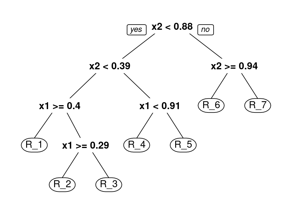
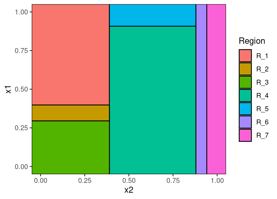
The top of the tree diagram is the root node. Each descendant to the left and right are child nodes, until the final nodes shown in ellipses which are leaves representing a region \(\mathcal{R}_j \subset \mathcal{X}\). Those parts of feature space represented by each leaf region are coloured on the second plot. We define the depth of a node to be the length of the path from the root to the node, so the node “x1 < 0.91” is at depth 2. We define the height of the tree to be the maximum over all depths, so the tree above has height 4.
The binary partitioning depicted here is along axis parallel splits, though that need not be true in general. For example, the \(j\)-th split could be of the form \(\vec{x}^T \vecg{\alpha}_j < c_j\) leading to non-axis parallel hyperplanes separating regions, or \(\| \vec{x} - \vecg{\alpha}_j \|_2 < c_j\) leading to spheres and their complement, or indeed anything that separates the remaining space in two. However, axis parallel splits are by far the most common and computationally tractable choice and leads to a partition comprised of hyper-rectangles. Hereinafter we restrict ourselves to only this setting, but see §6.1.6 for further reading.
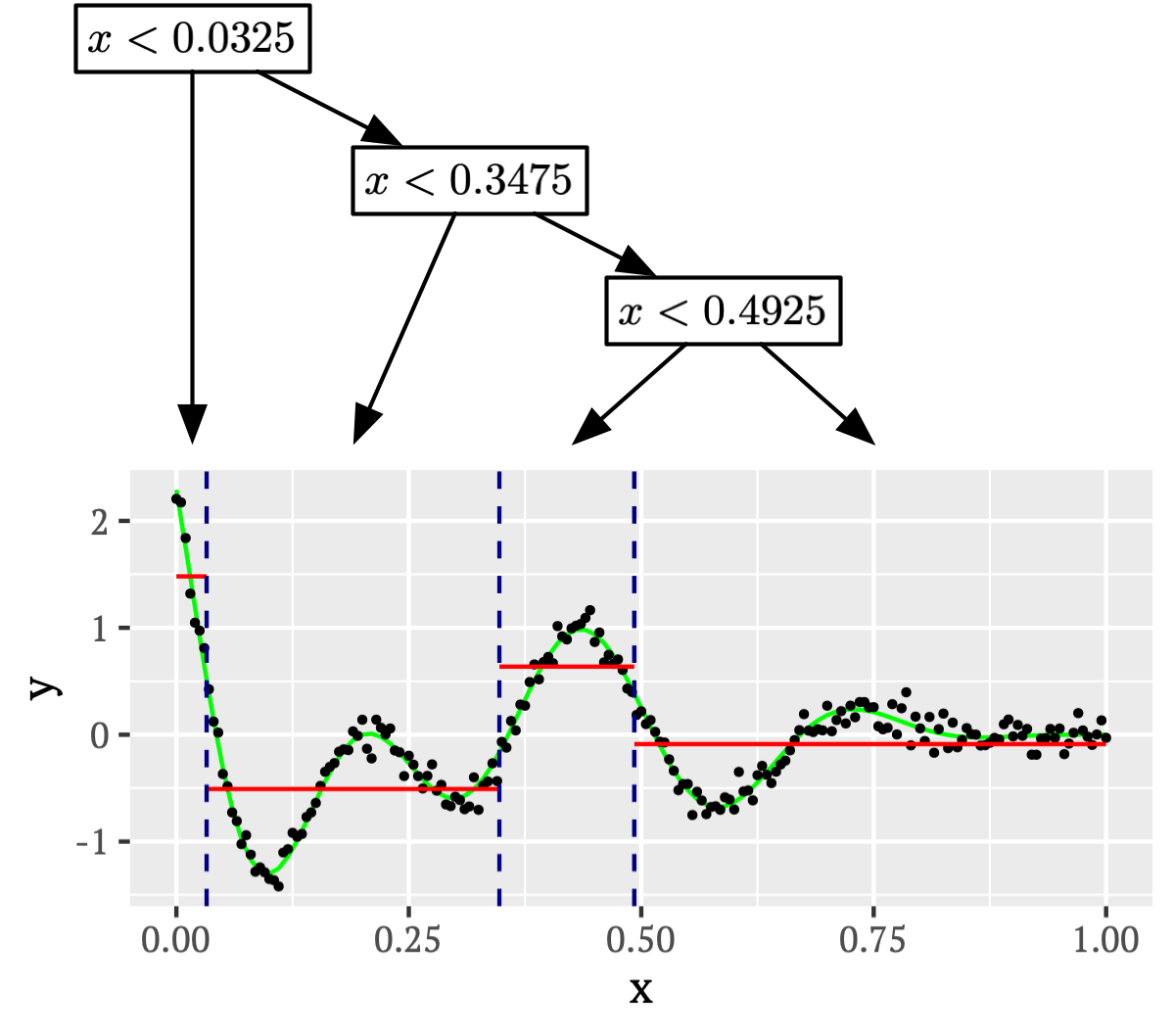
Tree methods aim to construct a partition of the feature space based on the observed data and to assign predicted responses to each region, be those labels in the classification setting, or numeric in the regression setting. For example, consider the toy example of 1-dimensional feature space regression depicted below, together with a tree representation which results in a piecewise constant functional fit:
The value assigned in each region will typically be set by empirical risk minimisation, thus matching the Bayes optimal predictor, in the case above selecting the mean of all response values within each region to minimise squared loss.
Therefore, given a tree, performing prediction is quite straightforward and the decisions which lead to a particular prediction are clear. However, a little thought reveals we are immediately presented with three problems when pondering how to construct such a tree:
if we have \(\vec{x}_i \ne \vec{x}_j \ \forall\,i \ne j\) then clearly it it possible to build a tree which completely segregates each observation into its own region, potentially leading to over-fitting (this situation bears a passing resemblance to 1-nearest neighbour).
there are infinitely many trees which would provide identical training error (and indeed infinitely many trees which would provide identical test error for hold-out) in the setting in (i) when the feature space is continuous.
assume we perhaps mitigate this by growing only to a fixed height \(L\), then there are still \(\sum_{\ell=0}^{L-1} 2^\ell = 2^L-1\) nodes in the tree, each splitting on one of \(d\) variables. Thus, jointly optimising the tree requires \(O\left( d(2^L-1) \right)\) operations per iteration of optimisation.
The “ideal” optimum tree is essentially out of reach and indeed can be proven to generally be computationally infeasible (Hyafil and Rivest, 1976), leading to a profusion of alternatives which attempt to approximate the optimal tree.
Probably the earliest examples of tree methods developed specifically for predictive purposes are Belson (1959) and Morgan and Sonquist (1963), where the analysis of survey data are considered. Nearly all the approaches which gained traction and remain popular today take a so-called “greedy search” approach to the tree building problem: that is, fixing node by node from the root down rather than attempting to simultaneously solve the whole tree. Murthy and Salzberg (1995) empirically show greedy search consistently achieves near optimal tree performance.
The most common tree algorithms in use today following this approach are CART (Breiman et al., 1984) and C4.5 (Quinlan, 1993) (an extension of ID3 (Quinlan, 1986)), or slight variations on them. We will focus on CART, this being the method closest to the implementations in both R (R Core Team, 2021) and Scikit-learn (Pedregosa et al., 2011).
There are many excellent intuitive descriptions of CART already (Hastie et al., 2009; James et al., 2013; Murphy, 2012) which you may want to read. Fewer resources develop a formal notation and description, so we proffer an attempt in that direction in the following two subsections. The intuitive or formal approach will appeal to different people, so feel free to use the above textbook resources instead of §6.1.1 and §6.1.2 if you prefer.
6.1.1 Binary tree notation
We first need to formalise our tree notation before we can define the CART algorithm.
Let \(\mathcal{R}_j^{(\ell)}\) denote the region specified by the \(j\)-th node at depth \(\ell\), for \(\ell \in \{1, 2, \dots\}\) and \(j \in \{ 0, \dots, 2^\ell-1 \}\). For example, at depth \(\ell=1\) there are two nodes and \(\mathcal{R}_0^{(1)} \cup \mathcal{R}_1^{(1)} = \mathcal{X}\).
We index \(j\) from \(0\) because it is useful to replace the double index \(\ell, j\) by a single vector index containing the \(\ell\) digit binary expansion of \(j\). In other words, noting that \(5_{10} \equiv 101_{2}\) we impose the notational equivalence \(\mathcal{R}_5^{(4)} \equiv \mathcal{R}_{0101}\), the superscript thus being unnecessary since the number of digits implies the depth. The utility of this binary notation becomes evident when visualised:
Thus, all children and deeper descendents of \(\mathcal{R}_{0}\) are indexed starting with the number 0 on the left half of the tree. In general, all descendents of a node are immediately identifiable as they have a strictly longer index which starts with the same binary string.
Now we can define a route through the tree to depth \(\ell\) by a vector \(\vecg{\tau}_\ell = (\tau_{\ell1}, \dots, \tau_{\ell\ell})\) with \(\tau_{\ell i} \in \{0,1\}\), where \(\tau_{\ell i}=0\) denotes taking the left branch when moving from depth \(i-1\) to \(i\), and \(\tau_{\ell i}=1\) denotes taking the right branch. Then \(\mathcal{R}_{\vecg{\tau}_\ell}\) indicates the region defined by the node reached along that route.
Given a region \(\mathcal{R}_{\vecg{\tau}_\ell}\) at depth \(\ell\), by obvious extension this node is split into two further regions \(\mathcal{R}_{\vecg{\tau}_\ell 0}\) and \(\mathcal{R}_{\vecg{\tau}_\ell 1}\) at depth \(\ell+1\), with \(\mathcal{R}_{\vecg{\tau}_\ell 0} \cap \mathcal{R}_{\vecg{\tau}_\ell 1} = \emptyset\) and \(\mathcal{R}_{\vecg{\tau}_\ell 0} \cup \mathcal{R}_{\vecg{\tau}_\ell 1} = \mathcal{R}_{\vecg{\tau}_\ell}\).
This notation is appropriate for any binary tree, but we are interested in trees arising from axis parallel splits, as discussed earlier. Therefore, with each non-leaf node we associate a split index \(i_{\vecg{\tau}_\ell}\) and split value \(s_{\vecg{\tau}_\ell}\) which give the dimension and location respectively at which this node is sub-divided into its left and right children.
Let us define region splitting functions, which create a binary partition in some region \(\mathcal{R}\) on dimension \(i\) at split value \(s\) by,
\[\begin{align*} \overleftarrow{\mathcal{X}}(\mathcal{R}, i, s) &:= \{ \vec{x} \in \mathcal{R} : x_i \le s \} \\ \overrightarrow{\mathcal{X}}(\mathcal{R}, i, s) &:= \{ \vec{x} \in \mathcal{R} : x_i > s \} \end{align*}\]Then we have the following recursive definition,
\[\begin{align*} \mathcal{R}_{\vecg{\tau}_\ell 0} &:= \overleftarrow{\mathcal{X}}(\mathcal{R}_{\vecg{\tau}_\ell}, i_{\vecg{\tau}_\ell}, s_{\vecg{\tau}_\ell}) \\ \mathcal{R}_{\vecg{\tau}_\ell 1} &:= \overrightarrow{\mathcal{X}}(\mathcal{R}_{\vecg{\tau}_\ell}, i_{\vecg{\tau}_\ell}, s_{\vecg{\tau}_\ell}) \end{align*}\]The recursive definition is completed by defining, for the empty set \(\emptyset\), that \(\mathcal{R}_\emptyset := \mathcal{X}\). Thus, a tree is fully defined by this recursion and the collection of split indices and values \(i_{\vecg{\tau}_\ell}\) and \(s_{\vecg{\tau}_\ell}\).
Therefore, we denote a tree by the collection \(\mathcal{T}\) consisting of pairs \((i_{\vecg{\tau}_\ell}, s_{\vecg{\tau}_\ell})\). The number of such pairs, \(|\mathcal{T}|\), is then the total number of nodes in the tree. We define \(\|\mathcal{T}\|_\Lambda\) to be the total number of leaf nodes in the tree (which is a direct measure of model complexity since it is the number of regions into which the tree splits \(\mathcal{X}\)).
Note the above is all easily extended to categorical variables by specifying a split set, instead of a split value, which contains the labels that go to the left child, with the complement going right.
6.1.2 CART
Given the notation defining an abstract binary tree structure with axis parallel splits, we turn to the problem of constructing such a tree on the basis of observed data. This amounts to learning the split indices and values.
We need one final piece of notation to relate the tree structure with the regions where data falls within that structure. To denote this, let the non-calligraphic versions of \(\mathcal{X}\) and \(\mathcal{R}\), \(X\) and \(R\) respectively, denote the set of observations in the corresponding region. For example,
\[ \overleftarrow{X}(\mathcal{R}, i, s) := \left\{ (\vec{x}, y) : (\vec{x}, y) \in \mathcal{D}, \vec{x} \in \overleftarrow{\mathcal{X}}(\mathcal{R}, i, s) \right\} \]
and thus \(R_{\vecg{\tau}_\ell 0} := \overleftarrow{X}(\mathcal{R}_{\vecg{\tau}_\ell}, i_{\vecg{\tau}_\ell}, s_{\vecg{\tau}_\ell})\). Similarly for \(\overrightarrow{X}\) and \(R_{\vecg{\tau}_\ell 1}\).
The CART algorithm is then a recursively grows a tree structure from the root node as follows.
Tree building: Initially, we start with \(\mathcal{T}=\emptyset\). Then, taking \(\ell=1\) we add \(\vecg{\tau}_1 = (0)\) and \(\vecg{\tau}_1 = (1)\) to a collection \(\mathcal{S}\) of indices yet to be solved.
Now select and remove the first \(\vecg{\tau}_\ell \in \mathcal{S}\) and proceed for this node index to solve for \(i_{\vecg{\tau}_\ell}\) and \(s_{\vecg{\tau}_\ell}\) as the arguments jointly minimising,
\[ \arg\min_{i,s} \left[ C\left(\overleftarrow{X}(\mathcal{R}_{\vecg{\tau}_\ell}, i, s)\right) + C\left(\overrightarrow{X}(\mathcal{R}_{\vecg{\tau}_\ell}, i, s)\right) \right] \]
subject to the constraint that \(|\overleftarrow{X}(\mathcal{R}_{\vecg{\tau}_\ell}, i, s)| > 0\) and \(|\overrightarrow{X}(\mathcal{R}_{\vecg{\tau}_\ell}, i, s)| > 0\) — if no split satisfies these constraints, select the next index from \(\mathcal{S}\) to be solved and move on. \(C(\cdot)\) is some cost function measuring the dissimilarity between response values in a set of data (see below). The action then taken depends on the stopping criterion (see below). If,
the stopping criterion is not triggered, then:
- \((i_{\vecg{\tau}_\ell}, s_{\vecg{\tau}_\ell})\) is added to \(\mathcal{T}\); and
- \(\vecg{\tau}_{\ell+1} = (\tau_{\ell 1}, \dots, \tau_{\ell \ell}, 0)\) and \(\vecg{\tau}_{\ell+1} = (\tau_{\ell 1}, \dots, \tau_{\ell \ell}, 1)\) are added to \(\mathcal{S}\).
the stopping criterion is triggered then discard \(i_{\vecg{\tau}_\ell}\) and \(s_{\vecg{\tau}_\ell}\), resulting in \(\mathcal{R}_{\vecg{\tau}_\ell}\) becoming a leaf on that branch.
Now continue to grow the tree by selecting the next index from \(\mathcal{S}\) to be solved, until there are no unsolved indices in \(\mathcal{S}\), at which point \(\mathcal{T}\) represents the fully constructed tree.
Cost functions: Note the cost function is a function on a set of observations, say \(R \subset \mathcal{D}\), falling within a proposed region, \(\mathcal{R} \subset \mathcal{X}\). Since trees make the same prediction for all observations falling in a leaf region, the purpose of the cost function is to measure how dissimilar training data responses are: for a region to be a good candidate for a new tree node all responses should be as alike as possible. The most common costs include:
Mean square error (regression), \[C(R) := \sum_{(\vec{x}, y) \in R} (y - \bar{y})^2\] where \(\bar{y} = \frac{1}{|R|} \sum_{(\vec{x}, y) \in R} y\)
Misclassification rate (classification) \[C(R) := \sum_{(\vec{x}, y) \in R} \bbone(y \ne \hat{y})\] where \(\hat{y}\) is the most frequently occurring label in the set \(R\).
Entropy/deviance (classification) \[C(R) := \sum_{g=1}^G \hat{p}_g \log \hat{p}_g\] where \(\hat{p}_g\) is the empirical proportion of label \(g\) in the set \(R\).
Gini index (classification) \[C(R) := \sum_{g=1}^G \hat{p}_g (1-\hat{p}_g)\] where \(\hat{p}_g\) is the empirical proportion of label \(g\) in the set \(R\).
All these cost functions aim to achieve so-called node purity, whereby splits lead to very similar response values \(y\) among the observations contained in each region.
Stopping criterion: In theory one could grow a tree until every leaf contains only a single observation. However, this would lead to massive overfitting. Consequently, some stopping criterion is usually employed. These include:
Imposing a complexity parameter which specifies the minimum amount by which a split must reduce the cost. That is, if the cost of the node being split minus the combined cost of the two child nodes does not exceed a complexity parameter then the split is prevented. (
cpargument inrpartR package)Apriori specification a height for the tree, such that any split which would result in new nodes with depth exceeding the set height is prevented. (
maxdepthargument inrpartR package)Selecting a limit on the minimum number of observations that can fall inside a node. That is, if a split results in either child node having too few observations then it is prevented. (
minsplitandminbucketarguments give two ways to set this inrpartR package, see?rpart.control)
However, a fundamental problem with stopping criterion is that by not allowing the tree to grow sufficiently we may end up missing important structure that would only be revealed after further splits.
The complexity parameter approach feels perhaps most sensible, founded as it is in some measurable performance quantity. However, it is not hard to construct examples which cause it to fail. Consider a data generating process that resembles a Battenberg Cake (or the corner of a chess board):
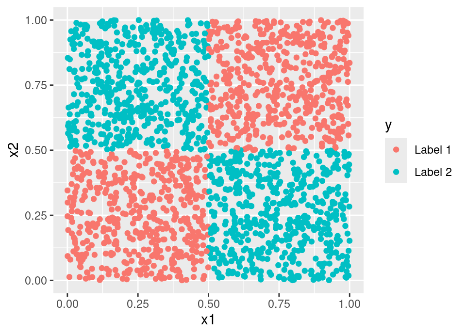
Then any axis parallel split will result in negligible cost reduction under any classification cost. Therefore, a complexity parameter stopping rule would refuse to make any splits, despite the fact the data set can be perfectly predicted by a binary tree structure. Indeed, this also provides a counter-example which proves trees grown via stopping rule are not universally consistent.
See the next sub-section for a better approach.
The following live code uses the rpart (Therneau and Atkinson, 2019) package to build a decision tree for the penguins data. The arguments cp = -1, minbucket = 1, minsplit = 1 to the function will cause the tree to fit a fully grown tree to purity, by disabling the complexity parameter and allowing single observation leaves (the tree height is already maximal by default in rpart). You can adjust these parameters to observe the effect of stopping rules.
# Things to explore:
#   - changing value of k on line 15
#   - using a different distance metric on line 16
#   - alter prediction point values on lines 19-20

# Package containing CART algorithm
library("rpart")

# Load data
data(penguins, package = "palmerpenguins")

# Fit tree
fit.tree <- rpart(species ~ bill_length_mm + bill_depth_mm,
                  penguins,
                  cp = -1, minbucket = 1, minsplit = 1)

# Example prediction point (shown as a white cross on plot)
new.pt <- data.frame(bill_length_mm = 59,
                     bill_depth_mm = 17)
predict(fit.tree, new.pt)

# Plot packages
library("ggplot2")
library("ggnewscale")

# Construct a hexagons grid to plot prediction regions
hex.grid <- hexbin::hgridcent(80,
                              range(penguins$bill_length_mm, na.rm = TRUE),
                              range(penguins$bill_depth_mm, na.rm = TRUE),
                              1)
hex.grid <- data.frame(bill_length_mm = hex.grid$x,
                       bill_depth_mm  = hex.grid$y)

# Get KNN vote predictions at the hex grid centres
hex.grid <- cbind(hex.grid,
                  predict(fit.tree, hex.grid))

# Construct a column of colourings based on Maxwell's Triangle
hex.grid$col <- apply(hex.grid[,3:5], 1, function(x) {
  x <- x/max(x)*0.9
  rgb(x[1],x[2],x[3])
})
all.cols <- unique(hex.grid$col)
names(all.cols) <- unique(hex.grid$col)

# Generate plot showing training data, decision regions, and new.pt
ggplot() +
  geom_hex(aes(x = bill_length_mm,
               y = bill_depth_mm,
               fill = col,
               group = 1),
           data = hex.grid,
           alpha = 0.7,
           stat = "identity") +
  scale_fill_manual(values = all.cols,
                    guide = "none") +
  new_scale("fill") +
  geom_point(aes(x = bill_length_mm,
                 y = bill_depth_mm,
                 fill = species),
             data = penguins,
             pch = 21) +
  scale_fill_manual("Species",
                    values = c(Adelie = "red",
                               Chinstrap = "green",
                               Gentoo = "blue")) +
  geom_point(aes(x = bill_length_mm,
                 y = bill_depth_mm),
             col = "white",
             pch = 4,
             data = new.pt)
6.1.3 Tree pruning
An alternative approach to mitigate overfitting uses so-called pruning, whereby a large tree is grown and then “pruned” by shortening certain branches. There are many ways one might select branches to prune and an overview of many early methods aiming to improve generalisation performance is provided by Mingers (1989). Beyond this, one may need a simpler pruned tree representation and seek a more compact/interpretable representation of a tree that already generalises well without sacrificing too much of the performance (Bohanec and Bratko, 1994).
More precisely, pruning corresponds to identifying one or more non-leaf nodes for which one wishes to remove all descendents, resulting in them becoming leaf nodes. In terms of the notation in this Chapter, the operation of pruning \(\mathcal{T}\) back to a particular node with index \(\vecg{\tau}_\ell\) is defined by:
\[\rho(\mathcal{T}, \vecg{\tau}_\ell) := \mathcal{T} \setminus \{ (i_{\vecg{\epsilon}_k}, s_{\vecg{\epsilon}_k}) : k \ge \ell \text{ and } \tau_{\ell i} = \epsilon_{k i} \ \forall\, i \in \{1, \dots, \ell\} \}\]
The process is repeated to prune to each node desired.
Cost-complexity pruning: We describe only the standard cost-complexity pruning of Breiman et al. (1984) here. This starts with a full tree and creates a nested sequence of sub-trees with minimally increasing apparent error (normalised by the change in tree complexity), then selecting the ‘best’ sub-tree on held-out data.
Recall (§3.4.1) that the apparent error is the estimated generalisation error using the training data, \(\widehat{\text{Err}}\). We will extend the notation to \(\widehat{\text{Err}}(\mathcal{T})\) to make clear what particular tree is being evaluated in the following.
First, a large tree is fitted, \(\mathcal{T}_0\), with either no stopping criterion or one with very permissive stopping criterion hyperparameters. Then, we prune tree \(\mathcal{T}_i\) to a sub-tree \(\mathcal{T}_{i+1}\) by first identifying which node to prune:
\[\vecg{\tau}_\ell = \arg\min_{\vecg{\epsilon}_k} \frac{\widehat{\text{Err}}(\rho(\mathcal{T}_i, \vecg{\epsilon}_k)) - \widehat{\text{Err}}(\mathcal{T}_i)}{\|\mathcal{T}_i\|_\Lambda - \|\rho(\mathcal{T}_i, \vecg{\epsilon}_k)\|_\Lambda}\]
and then define \(\mathcal{T}_{i+1} = \rho(\mathcal{T}_i, \vecg{\tau}_\ell)\). This recursively defines a collection of nested sub-trees, \(\mathcal{T}_0, \mathcal{T}_1, \dots\). We then use held-out data to choose one of the trees.
Notice that the reduction in apparent error from this pruning operation is:
\[\begin{align*} \alpha_i &= \frac{\widehat{\text{Err}}(\rho(\mathcal{T}_i, \vecg{\tau}_\ell)) - \widehat{\text{Err}}(\mathcal{T}_i)}{\|\mathcal{T}_i\|_\Lambda - \|\rho(\mathcal{T}_i, \vecg{\tau}_\ell)\|_\Lambda} \\ %\implies \widehat{\text{Err}}(\rho(\mathcal{T}_i, \vecg{\tau}_\ell)) &= \widehat{\text{Err}}(\mathcal{T}_i) + \alpha_i \left( \|\mathcal{T}_i\|_\Lambda - \|\rho(\mathcal{T}_i, \vecg{\tau}_\ell)\|_\Lambda \right) \\ \implies \widehat{\text{Err}}(\rho(\mathcal{T}_i, \vecg{\tau}_\ell)) + \alpha_i \|\rho(\mathcal{T}_i, \vecg{\tau}_\ell)\|_\Lambda &= \widehat{\text{Err}}(\mathcal{T}_i) + \alpha_i \|\mathcal{T}_i\|_\Lambda \end{align*}\]As such, we can see tree pruning as defining a regularised path through tree space, therefore linking this approach to the statistical theory of regularisation used in models like the lasso and ridge regression (see High-dimensional Statistics APTS module (Loh and Yu, 2025)).
Such a procedure would overcome the issue described in the previous sub-section in the ‘Battenburg Cake’ example, so long as the tree is forced to make an initial split.
6.1.4 Theory
There are quite general conditions provided for the consistency of tree methods in the classification and density estimation (Lugosi and Nobel, 1996), as well as regression cases (Nobel, 1996). However, we will not go into detail here as it requires introducing substantial additional content to state the conditions. For a longer form discussion of tree theory in the classification setting, see Chapters 20 and 21 of Devroye et al. (1996).
6.1.5 Discussion
Tree methods are often appealing in applications, because they mimic the decision making processes often employed by humans. For example, the following is a real decision tree used by A&E doctors to decide the bed type to assign for cardiac patients:
Being able to learn such trees from data, controlling their complexity with pruning, also means they are still used in many projects today where often such rules must be executed by humans rather than by computer. In these settings, easy interpretation is also critical, which trees offer.
However, trees are not without their drawbacks. Trees really struggle to represent additive relationships so may underperform even misspecified standard linear models where there is an additive relationship. Additionally, trees tend to be extremely high variance estimators (Dietterich and Kong, 1995). The following live code block performs a simple simulation experiment to demonstrate this. We simulate 50 observations from the model \(\pi_X \sim \text{Unif}\left([0,1]^2\right)\) and \(\pi_{Y \given X=\vec{x}} \sim \text{N}(\mu = x_1^2 + x_2^2, \sigma = 0.1)\), then fit both a standard linear model \(\vec{x}^T \vecg{\beta}\) and a tree \(\mathcal{T}\) many times, computing a Monte Carlo approximation of the true generalisation error. Then, repeating this process many times we can get an estimate of the variance of generalisation error. Note that strictly speaking both the linear model and the tree are misspecified in this setting.
library("rpart")
# library("randomForest")

set.seed(212)

mk.data <- function(n = 50) {
  X <- data.frame(x1 = runif(n),
                  x2 = runif(n))
  X$y <- X$x1^2 + X$x2^2 + rnorm(n, sd = 0.1)
  X
}

n.it <- 500
mse.tree <- rep(0, n.it)
# mse.bag <- rep(0, n.it)
mse.lm <- rep(0, n.it)

for(i in 1:length(mse.tree)) {
  # Generate a new data set of size 50
  X.tr <- mk.data()

  # Fit a tree and linear model to this training data
  fit.tree <- rpart(y~., X.tr)
  # fit.bag <- randomForest(y~., X.tr, mtry = 2)
  fit.lm <- lm(y~., X.tr)

  # Generate a testing data set
  X.te <- mk.data(1000)

  # Compute generalisation error and store
  mse.tree[i] <- mean((predict(fit.tree, X.te) - X.te$y)^2)
  # mse.bag[i]  <- mean((predict(fit.bag, X.te) - X.te$y)^2)
  mse.lm[i]   <- mean((predict(fit.lm, X.te) - X.te$y)^2)
}

# Expected generalisation error
mean(mse.tree)
# mean(mse.bag)
mean(mse.lm)

# Standard deviation of generalisation error
sd(mse.tree)
# sd(mse.bag)
sd(mse.lm)
Running the above code, you can observe that the linear model is not only more accurate on average, but also has much lower variance.
6.1.6 Further reading
Axis parallel splits are not the only approach. When introducing axis-parallel trees in Breiman et al. (1984), they also suggested an early direct search method to find hyperplane splits, \(\vec{x}^T \vecg{\alpha}_j < c_j\). Heath et al. (1993) coined the term “oblique decision tree” to describe such splits and provided a simulated annealing algorithm to find them. This was improved upon in Murthy et al. (1994). There is limited theory on the performance of oblique trees, but recent consistency results are provided by Zhan et al. (2025). If you would like to play with these types of tree (and forests of them), see the R package ODRF (Liu and Xia, 2025).
Everything presented above placed accurate prediction as paramount and is therefore in keeping with the machine learning disposition of this course. However, there is a different and more statistical approach to tree building, where statistical significance plays a role to “distinguish between a significant and an insignificant improvement” (Mingers, 1987). Hothorn et al. (2006) is a recent example of tree building methodology in this tradition.
6.1.7 Software
The function rpart::rpart (Therneau and Atkinson, 2019) follows the CART algorithm very closely, and provides other tools for working with single trees. However, the plotting functionality is rather basic, so I recommend using the rpart.plot package (Milborrow, 2021) which has excellent and attractive plotting features.
The party R package implements the statistical tree building approach of Hothorn et al. (2006).
If your research requires using tree data structures, then the data.table package (Glur, 2020) provides a clean modern interface for this, independent of the context of CART, statistical machine learning or any other discussion here.
6.2 Bagging
As discussed above, trees have many appealing properties, but a very serious Achilles heel: they are a very high variance estimator. Breiman (1996) introduced the beautifully simple yet effective concept of bagging in an effort to combat this drawback.
Definition 6.2 (Bagged estimator) Let \(\hat{f}(\cdot \given \mathcal{D})\) represent some model (eg trees) fitted to a particular data set \(\mathcal{D}\). Then \(\hat{f}\) can be turned into a bagged estimator by repeatedly fitting the model to bootstrap resamples of the data, taking the average of all the fitted models. The model used to refit repeatedly is called the base learner.
That is, draw \(B\) new samples of size \(|\mathcal{D}|\) with replacement from \(\mathcal{D}\), giving \(\mathcal{D}^{\star 1}, \dots, \mathcal{D}^{\star B}\) and let:
\[\hat{f}^\text{bag}(\vec{x}) := \frac{1}{B} \sum_{b=1}^B \hat{f}(\vec{x} \given \mathcal{D}^{\star b})\]
The name “bagging” is an abbreviation of Bootstrap AGGregatING.
It may not be immediately obvious why this procedure is sensible and is often difficult to analyse bootstrap procedures. To simplify matters but provide an intuition, imagine that we know \(\pi_{XY}\) precisely and can draw samples from it, then a theoretically idealised bagged estimator is:
\[\hat{f}^\text{bag}(\vec{x}) = \mathbb{E}_{D_n} \left[ \hat{f}(\vec{x} \given D_n) \right]\]
Notice that this is the quantity that the bootstrap procedure is empirically approximating. Then, thinking of the regression setting with squared loss, let us take an expectation over training sets of the squared loss,
\[\begin{align*} \mathbb{E}_{D_n} \left[ \left( y - \hat{f}(\vec{x} \given D_n) \right)^2 \right] &= y^2 - 2 y \, \mathbb{E}_{D_n} \left[ \hat{f}(\vec{x} \given D_n) \right] + \mathbb{E}_{D_n} \left[ \hat{f}(\vec{x} \given D_n)^2 \right] \\ &\ge y^2 - 2 y \, \mathbb{E}_{D_n} \left[ \hat{f}(\vec{x} \given D_n) \right] + \mathbb{E}_{D_n} \left[ \hat{f}(\vec{x} \given D_n) \right]^2 \\ &= \left( y - \mathbb{E}_{D_n} \left[ \hat{f}(\vec{x} \given D_n) \right] \right)^2 \\ &= \left( y - \hat{f}^\text{bag}(\vec{x}) \right)^2 \end{align*}\]The inequality following since \(\mathbb{E}[X^2] \ge \mathbb{E}[X]^2\). If we now take a further expectation with respect to \(\pi_{Y \given X=\vec{x}}\), then we have the expected prediction error (§3.6), giving
\[\mathbb{E}_{Y \given X=\vec{x}} \left[ \mathbb{E}_{D_n} \left[ \left( Y - \hat{f}(\vec{x} \given D_n) \right)^2 \right] \right] \ge \mathbb{E}_{Y \given X=\vec{x}} \left[ \left( Y - \hat{f}^\text{bag}(\vec{x}) \right)^2 \right]\]
Consequently, this idealised bagged estimator will have lower expected prediction error than the base learner estimate built only on each training data set. Indeed, it is lower by precisely
\[\mathbb{E}_{D_n} \left[ \hat{f}(\vec{x} \given D_n)^2 \right] - \mathbb{E}_{D_n} \left[ \hat{f}(\vec{x} \given D_n) \right]^2 = \text{Var}_{D_n}\left( \hat{f}(\vec{x} \given D_n) \right)\]
In other words, the bagging estimator is most effective when the variance of the base learner is high with respect to the training sample. This is exactly the situation with trees, which is why bagging is most often deployed with tree models. Note that this derivation is true for any model though, and bagging has been shown for example to improve \(k\)-nearest neighbour models too (though for knn the bootstrap resample size must be at most 69% of \(|\mathcal{D}|\) (Hall and Samworth, 2005)).
Of course, we cannot hope to achieve all the gains available since we can only approximate \(\mathbb{E}_{D_n}\) by bootstrapping, but this has been observed to perform well in a wide array of settings.
Classification: A similar argument can be made for classification problems (see Breiman, 1996 for full details). However, care is required in exactly how the individual models are combined. There are two reasonable ways one might define the bagged estimate: first is to simply average the Bayes optimal predictors of each tree:
\[\begin{align*} \hat{f}_j^\text{bag}(\vec{x}) &= \frac{1}{B} \sum_{b=1}^B \bbone\left\{ \arg \max_k \left( \hat{f}_k\left(\vec{x} \given \mathcal{D}^{\star b}\right) \right) = j \right\} \\ \hat{f}^\text{bag}(\vec{x}) &= (\hat{f}_1^\text{bag}(\vec{x}), \dots, \hat{f}_g^\text{bag}(\vec{x})) \end{align*}\]This will produce a good classifier under 0-1 loss, but one should be aware that even if every tree is perfectly calibrated then this estimator will be completely uncalibrated. For example, if the true \(p_\ell(\vec{x}) = 0.8\), for some response label \(\ell\), and all trees are close to well calibrated at this probability, then the above procedure ends up assigning a bagged probability of 1 to label \(\ell\). This is perhaps not a concern if you do not require a probabilistic estimate.
However, when bagging classifiers and seeking a probabilistic estimate it is important to directly average the estimated probabilities:
\[\hat{f}_j^\text{bag}(\vec{x}) = \frac{1}{B} \sum_{b=1}^B \hat{f}_k\left(\vec{x} \given \mathcal{D}^{\star b}\right)\]
A nice additional property proved in the same paper is that as long as the constituent models are order-correct (that is, on average the most prevalent class is identified), then even if it is suboptimal the bagging procedure transforms the collection into a near optimal predictor. However, caveat emptor … bagging a poor classifier base model will in fact make it worse, not better, unlike the regression case.
6.2.1 Out of bag error
Note that when performing bootstrap resampling, the sampling with replacement of a data set of the same size means that clearly not every observation will be included on each sample. Indeed, for any given observation:
\[\begin{align*} &\mathbb{P}\left( (\vec{x}_i, y_i) \in \mathcal{D}^{\star b} \right) \\ &\qquad = 1 - \mathbb{P}\left( (\vec{x}_i, y_i) \notin \mathcal{D}^{\star b} \right) \\ &\qquad = 1 - \mathbb{P}\left((\vec{x}_1^{\star b}, y_1^{\star b}) \ne (\vec{x}_i, y_i) \cap \dots \cap (\vec{x}_n^{\star b}, y_n^{\star b}) \ne (\vec{x}_i, y_i)\right) \\ &\qquad = 1 - \prod_{j=1}^n \mathbb{P}\left((\vec{x}_j^{\star b}, y_j^{\star b}) \ne (\vec{x}_i, y_i)\right) \qquad \text{by indep sampling with replacement} \\ &\qquad = 1 - \left(1 - \frac{1}{n}\right)^n \\ &\qquad \approx 1 - e^{-1} \approx 0.632 \end{align*}\]In other words, approximately \(1-0.632=36.8\%\) of observations are not used when fitting any single bootstrap resample. Likewise, for a single observation, this means it does not appear in about 36.8% of the fitted models. This provides a powerful and simple method to assess the error of a bagged model without having to maintain a hold-out set, or to use cross-validation.
Definition 6.3 (Out Of Bag (OOB) error) The out of bag error of a bagged estimator is the estimated generalisation error where the bagged estimator varies computed using the bagged estimator consisting of only those models fitted to bootstrap resamples not containing the given observation.
More precisely, define \(\mathcal{B}_{-i} := \{ b : (\vec{x}_i, y_i) \notin \mathcal{D}^{\star b} \}\) to be the indicies of the bootstrap resamples not containing sample \(i\). Then, \[\hat{\mathcal{E}}_\text{OOB}\left(\hat{f}^\text{bag}\right) := \frac{1}{n} \sum_{i=1}^n \mathcal{L}\left( y_i, \frac{1}{|\mathcal{B}_{-i}|} \sum_{b \in \mathcal{B}_{-i}} \hat{f}\left(\vec{x}_i \given \mathcal{D}^{\star b}\right) \right)\]
The OOB error provides an excellent ‘online’ monitor of the algorithm: we can plot OOB error against the number of bootstrap resampled base learner models and look for the error curve to flatten. We know from later work which extended bagging (see next section) that it follows from the Strong Law of Large Numbers that bagging does in fact converge (Breiman, 2001b). The following is an example of a OOB error curve in a simulated example:
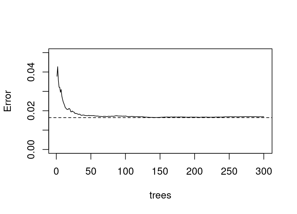
We can see that by 100 bootstrap resampled trees the error has become quite stable and is a rather good estimate of the true generalisation error of the full bagged model, which is shown by the dashed line (estimated by a large independent test sample).
Note that the OOB estimate is of course based, on average, on a bagged estimator consisting of just over a third as many models as the true estimator. Therefore, to have some confidence in OOB error we should in reality train well beyond the flattening of the error curve to be sure of stability in the error estimate with the size of bagged model.
Finally, given the discussion of Chapter 5 it is important to ask what exactly is estimated by the OOB error? The answer is, asymptotically, that OOB error converges to LOO cross validation (Hastie et al., 2009), so earlier commentary on that applies here (at least asymptotically).
6.2.2 Discussion
It would be hard to improve upon the conclusion in the original bagging paper, which vividly evokes a 16th-century proverb, so I simply quote it in summing up:
“Bagging goes a ways toward making a silk purse out of a sow’s ear, especially if the sow’s ear is twitchy. It is a relatively easy way to improve an existing method, since all that needs adding is a loop in front that selects the bootstrap sample and sends it to the procedure and a back end that does the aggregation. What one loses, with the trees, is a simple and interpretable structure. What one gains is increased accuracy.”
library("rpart")
library("randomForest")

set.seed(212)

mk.data <- function(n = 50) {
  X <- data.frame(x1 = runif(n),
                  x2 = runif(n))
  X$y <- X$x1^2 + X$x2^2 + rnorm(n, sd = 0.1)
  X
}

n.it <- 500
mse.tree <- rep(0, n.it)
mse.lm <- rep(0, n.it)
mse.bag <- rep(0, n.it)
oob.bag <- rep(0, n.it)

for(i in 1:length(mse.tree)) {
  # Generate a new data set of size 50
  X.tr <- mk.data()

  # Fit a tree and linear model to this training data
  fit.tree <- rpart(y~., X.tr)
  fit.lm <- lm(y~., X.tr)
  fit.bag <- randomForest(y~., X.tr, mtry = 2)
  oob.bag[i]  <- fit.bag$mse[length(fit.bag$mse)]

  # Generate a testing data set
  X.te <- mk.data(1000)

  # Compute generalisation error and store
  mse.tree[i] <- mean((predict(fit.tree, X.te) - X.te$y)^2)
  mse.lm[i]   <- mean((predict(fit.lm, X.te) - X.te$y)^2)
  mse.bag[i]  <- mean((predict(fit.bag, X.te) - X.te$y)^2)
}

# Expected generalisation error
mean(mse.tree)
mean(mse.lm)
mean(mse.bag)
mean(oob.bag)

# Standard deviation of generalisation error
sd(mse.tree)
sd(mse.lm)
sd(mse.bag)
sd(oob.bag)
6.3 Random Forests
The bagging estimator is just one of a whole class of estimators based on randomising the training data to create a so-called ensemble model comprised of many base learners. Other forms of randomisation include:
- instead of taking the best split when growing a tree, uniformly at random select among the best \(k\) splits (Dietterich, 2000), repeating many times and combine all the trees into an ensemble.
- instead of building a tree on the full space \(\mathcal{X}\), project all observations into a subspace consisting of only some dimensions and grow a tree in that space (Ho, 1998), again repeating many times and combining into an ensemble. Ho (1998) coined the phrase “decision forest” to describe this approach.
- in a similar spirit to the last bullet, consider a random subspace of features but where that subspace varies each time a new node is split (Amit and Geman, 1997) (in fact there is much more around engineered features in that paper specific to image recognition, but this is the core idea relevant to us).
Breiman (2001b) identified that the three above randomisation methods operating on features, and his earlier work on bagging which randomised through observations, could all be unified under a single framework he termed random forests. Indeed, a random forest (most broadly interpreted) is simply any model formed by an ensemble of randomised trees.
The original random forest algorithm combined randomisation from bagging (Breiman, 1996) and random subspaces at each split (Amit and Geman, 1997) for each tree, and is the method implemented in the randomForest R package (Liaw and Wiener, 2002). However, the framework and many of the results proved in the original paper apply in the much broader framework.
6.3.1 Theory
Breiman (2001b) provided several key insights into the theoretical behaviour of random forests.
Firstly, asymptotically as the number of trees increases, the error rate of the forest converges to the limiting value of the generalisation error for the particular set of randomised base learners feeding into the forest. Therefore, adding more trees will not cause a forest to overfit (NB obviously changing the randomised models feeding the forest will still change what that asymptotic error is!)
Secondly, the generalisation error can be bounded:
\[\mathcal{E} \le \frac{\bar{\rho} (1-S^2)}{S^2}\]
where \(S\) is how ‘strong’, and \(\bar{\rho}\) is how correlated, the randomised models feeding the forest are.
Informally, \(S\) is the expected excess probability of a randomised base learner predicting the correct response label: 1 means the model always predicts the correct label with certainty; near 1 implies correct prediction and that the next highest label probability was low; and near zero implies indecision in that the probability predicted for the wrong label was close to that of the correct one.
Informally, \(\bar{\rho}\) is how correlated the strength of individual randomised base learners feeding the forest are (averaged over the randomising mechanism). See Breiman (2001b) for the formal definitions which would require too much diversion to fully detail here.
This result indicates that the best forests are comprised of base learners which make confident correct decisions and which are very uncorrelated with one another. This helps to understand why random forests improve on bagging alone: taking random subspaces at each split further breaks the correlation between predictions made by individual trees. Of course, \(S\) and \(\bar{\rho}\) are inevitably linked and so tuning the randomising mechanism is likely to be necessary.
6.3.2 Software
The standard implementation of Breiman’s original random forest is in the randomForest package (Liaw and Wiener, 2002). A fantastic high performance modern implementation with full parallelisation built in is ranger (Wright and Ziegler, 2017)
6.4 Boosting
As we saw above, random forests depend in part on having strong base learners, otherwise one relies entirely on having extremely low correlation between learners to achieve good generalisation error. Well before the conception of random forests, Michael Kearns (1988) asked a now famous question in his machine learning class project: is it possible for weak learners be combined to create a strong learner with low bias? He termed this the “Hypothesis Boosting Problem”, and it is quite different to the random forest setting.
A few years later, the question was rigorously answered in the affirmative by Robert Schapire (1990), and another algorithm provided soon after by Freund (1995). However, these early approaches required apriori knowledge of the strength of the base learners making them hard to deploy. The first practical fully adaptive method was named AdaBoost and introduced in Freund and Schapire (1997), work which won the authors the Gödel Prize 6 years later.
At a high level, all boosting algorithms are founded on the idea of creating an ensemble classifier of \(B\) weak learners. We use \(\hat{F}^{(B)}(\cdot)\) to denote the ensemble model (this is a function, not a cdf!) comprised of individual contributions \(\hat{f}^{(b)}(\cdot)\),
\[\hat{F}^{(B)}(\vec{x}) = \sum_{b=1}^B \alpha_b \hat{f}^{(b)}(\vec{x})\]
which is iteratively built, with each successive weak base learner in the ensemble being specifically constructed to improve upon or correct errors of the previous ensemble members. These ideas led to a profusion of specific algorithms to address this iterative building process: we will describe AdaBoost first as the chronological original practical boosting algorithm, followed by a generic framework and references to high profile instances. In principle the base learner can usually be anything, but trees with quite constrained height are a very common choice (the height constraint making them weak learners).
Let \(\mathcal{T}_{(h)}\) denote the function space of all trees of height \(h\).
6.4.1 AdaBoost
The AdaBoost algorithm Freund and Schapire (1997) was developed for binary classification and in the following we take the response label to be \(\mathcal{Y} = \{-1, +1\}\). Additionally, AdaBoost assumes the weak learner \(\hat{f}^{(b)} : \mathcal{X} \to \{-1, +1\}\), that is, it does not return a probabilistic estimate.
We define weights, \(\vec{w} = (w_1, \dots, w_n)\), for each observation in \(\mathcal{D}\). Initially, we set \(w_i = 1/n \ \forall\, i\) and define the initial overall model \(\hat{f}(\vec{x}) = 0 \ \forall\, \vec{x}\in\mathcal{X}\). Then, we repeat for iterations \(b = 1,\dots,B\):
- Fit a tree to the weighted dataset according to the following loss \[ \hat{f}^{(b)} = \arg\min_{f \in \mathcal{T}_{(h)}} \sum_{\{ i : f(\vec{x}_i) \ne y_i \}} w_i \] That is, seek the tree of fixed height which minimises the total weight of misclassified observations.
- Compute the weighted error: \[ \varepsilon_b = \sum_{i=1}^n w_i \bbone\left\{ \hat{f}^{(b)}(\vec{x}_i) \ne y_i \right\}\]
- If \(\varepsilon \ge \frac{1}{2}\) then discard \(\hat{f}^{(b)}\) and terminate the algorithm. Otherwise, if \(\varepsilon < \frac{1}{2}\), then retain \(\hat{f}^{(b)}\) and set the coefficient of this weak learner to be \[\alpha_b = \frac{1}{2} \log \left( \frac{1-\varepsilon}{\varepsilon} \right)\] and update all observation weights as: \[w_i \leftarrow \frac{w_i \exp\left( -\alpha_b \hat{f}^{(b)}(\vec{x}_i) y_i \right)}{2 \sqrt{\varepsilon (1-\varepsilon)}}\]
Upon termination, we will have up to \(B\) weak learners \(\hat{f}^{(b)}\) together with coefficient weights \(\alpha_b\), leading to the full ensemble, \[\hat{F}(\vec{x}) = \sum_{b} \alpha_b \hat{f}^{(b)}(\vec{x})\] where the sign of the prediction indicates the label (ie a scoring classifier). If we terminate early due to \(\varepsilon_b \ge \frac{1}{2}\), this means we reached a point where the weak learner was no better than guessing and so adding further weak learners would not benefit the ensemble.
AdaBoost is designed to aggressively drive the training/apparent error down as quickly as possible. Indeed, the 0-1 training error of the ensemble is bounded, \[\widehat{\text{Err}} \le \prod_{b=1}^B \sqrt{1-4\left(\frac{1}{2}-\varepsilon_b\right)^2}\] Therefore, if each weak learner’s error rate was, for example no more than 40%, then the error would be bounded by \(0.98^B\), an exponentially fast decrease. In particular, if \(n\,\widehat{\text{Err}} < 1\), then not a single training observation would be misclassified, but this implies \[B > \frac{2 \log n}{\log \left(\left(1-4\left(\frac{1}{2}-\varepsilon_b\right)^2\right)^{-1}\right)}\] In other words, within \(O(\log n)\) iterations the training error will be zero. It is also possible to get quite generic bounds on the generalisation error of AdaBoost, for details see Schapire and Freund (2012), Chapter 4.
Breiman (1998) studied AdaBoost and related algorithm’s statistical behaviour (he calls boosting “arcing” and refers to AdaBoost as arc-fs throughout that paper). He examined bagging as an alternative to the minimised weighted fitting of \(\hat{f}^{(b)}\), showing that the variance reduction AdaBoost achieves is due to the adaptive resampling via weights. Also of particular interest, he notes that when AdaBoost is run far past the point at which training error reaches zero it continues to improve in out-of-sample generalisation error (and outperforms bagging methods), it typically being very rare to suffer overfitting. Later the same year, Bartlett et al. (1998) examined this phenomenon in detail, attributing it to boosting continuing to improve the margin (similarly defined to the random forest section) of classification prediction well past zero training error.
6.4.2 Boosting = greedy forward stagewise
An important paper from a statistician’s perspective is Friedman et al. (2000), which strips away much mystery surrounding AdaBoost. In this work they both extended AdaBoost to probabilistic base learners, \(\hat{f}^{(b)} : \mathcal{X} \to [0,1]\), and more importantly, they show that AdaBoost is in fact a form of forward stagewise regression estimator, fitting successively to residuals (a common technique in additive modelling known for some time in statistics) where the constituent model is optimising an exponential classification loss (recall § 3.3). These observations immediately opened the door to constructing boosting methods in much greater generality.
In fact, forward stagewise13 regression estimation is a particularly intuitive and simplified form to assist in developing an intuition for boosting, so for clarity we show the particular case of regression with square loss:
Set \(\varepsilon_i = y_i\) for \(i \in \{ 1, \dots, n \}\)
For \(b = 1,\dots,B\), iterate:
- Fit a model (eg tree) \(\hat{f}^{(b)}(\cdot)\) and multiplier \(\lambda_b\) to the response \(\varepsilon_1, \dots, \varepsilon_n\) as, \[\{ \hat{f}^{(b)}(\cdot), \lambda_b \} \leftarrow \arg\min_{f \in \mathcal{T}_{(h)}, \lambda_b\in\mathbb{R}} \sum_{i=1}^n \left( \varepsilon_i - \lambda_b \hat{f}^{(b)}(\vec{x}) \right)^2\]
- Update the residuals \[ \varepsilon_i \leftarrow \varepsilon_i - \lambda_b \hat{f}^{(b)}(\vec{x}) \quad \forall\ i \]
Output as final boosted model \[ \hat{F}^{(B)}(\vec{x}) = \sum_{b=1}^B \lambda_b \hat{f}^{(b)}(\vec{x}) \]
The main distinction is the lack of any weighting of observations to focus on difficult cases, and clearly least squares is only appropriate for regression. Therefore, Friedman et al. (2000) continue in their paper to develop LogitBoost, directly using the binomial log-likelihood as fitting criterion with observation weighting (now, we revert to the more standard \(\mathcal{Y} = \{0,1\}\)):
Let \(\vec{w}\) be weights for each observation in \(\mathcal{D}\), with \(w_i = 1/n \ \forall\, i\). Let the overall model \(\hat{f}(\vec{x}) = 0 \ \forall\, \vec{x}\in\mathcal{X}\), and initial probabilistic estimates \(p_i = \frac{1}{2} \ \forall\, i\).
For \(b = 1,\dots,B\), iterate:
- Compute weights and responses \[\begin{align*} w_i &= p_i(1-p_i) \\ z_i &= \frac{y_i - p_i}{p_i(1-p_i)} \end{align*}\]
- Fit \(\hat{f}^{(b)}(\cdot)\) by a weighted least-squares regression of \(z_i\) to \(x_i\) with weight \(w_i\).
- Update \(\hat{f}(\vec{x}) \leftarrow \hat{f}(\vec{x}) + \frac{1}{2}\hat{f}^{(b)}(\vec{x})\) and \(p_i \leftarrow \exp(\hat{f}(\vec{x}_i))/\left(\exp(\hat{f}(\vec{x}_i))+\exp(-\hat{f}(\vec{x}_i))\right)\)
Upon termination the full ensemble is \(\hat{F}^{(B)}(\vec{x}) = \sum_b \hat{f}^{(b)}(\vec{x})\) where the sign of the prediction indicates the class (ie a scoring classifier).
6.4.3 Gradient boosting machines
You may have found some of the forms of stagewise equations above quite reminiscent of gradient descent, where an estimate is updated by some scaled move. Recall, generic gradient descent to minimise a function \(g(\theta)\) takes a starting point \(\theta_0\) and iterates:
\[\theta_{i+1} = \theta_i - \gamma \, \nabla g(\theta) \Big|_{\theta = \theta_i}\]
where \(\nabla g(\theta) \Big|_{\theta = \theta_i}\) denotes the gradient of \(g\) evaluated at \(\theta = \theta_i\). We do not normally write it this way, but we could express the final value as \[\hat{\theta} = \theta_0 - \sum \gamma \, \nabla g(\theta) \Big|_{\theta = \theta_i}\] which now strongly evokes the form of boosted models, ie \(\gamma \leftrightarrow \alpha_b\) and \(\nabla g(\theta) \Big|_{\theta = \theta_i} \leftrightarrow \hat{f}^{(b)}(\vec{x})\)
Theoretical motivation: Friedman (2001) was first to develop a general boosting framework around gradient descent. This can be thought of as performing empirical risk minimisation via gradient descent directly in the function space of the base learner.
Let us denote the \(B\) term boosting estimate to be \(\hat{F}^{(B)}(\vec{x}) = \sum_{b=1}^B \alpha_b \hat{f}^{(b)}(\vec{x})\). Recall that the generalisation error for a general predictor \(F\) is:
\[\mathcal{E}\left( F \right) = \mathbb{E}_{XY} \mathcal{L}\left( Y, F(X) \right) = \mathbb{E}_{X} \left[ \mathbb{E}_{Y \given X = \vec{x}} \left[ \mathcal{L}\left( Y, F(\vec{x}) \right) \right] \right]\]
We can tackle this by minimising at each point \(\vec{x}\). That is, we want to minimize the inner expectation for each \(\vec{x}\), which we denote:
\[\mathcal{E}\left( F(\vec{x}) \right) := \mathbb{E}_{Y \given X} \mathcal{L}\left( Y, F(\vec{x}) \right)\]
Therefore, if we currently have ensemble total \(\hat{F}^{(B)}(\vec{x})\) and we want to add another member to the ensemble to reduce the generalisation error, we could think of this as a gradient descent step in the function space to which \(F\) belongs, to make \(\mathcal{E}\left( F(\vec{x}) \right)\) smaller:
\[\left.\hat{F}^{(B+1)}(\vec{x}) = \hat{F}^{(B)}(\vec{x}) - \gamma \nabla \mathcal{E}\left( F(\vec{x}) \right)\right|_{F(\vec{x}) = \hat{F}^{(B)}(\vec{x})}\]
We abbreviate the gradient term to \(\eta_B(\vec{x})\), which in full is:
\[\begin{align*} \eta_B(\vec{x}) := \nabla \mathcal{E}\left( F(\vec{x}) \right)\Big|_{F(\vec{x}) = \hat{F}^{(B)}(\vec{x})} &= \left.\frac{\partial\,\mathbb{E}_{Y \given X} \mathcal{L}\left( Y, F(\vec{x}) \right)}{\partial\,F(\vec{x})}\right|_{F(\vec{x}) = \hat{F}^{(B)}(\vec{x})} \\ &= \mathbb{E}_{Y \given X} \left[ \left.\frac{\partial\,\mathcal{L}\left( Y, F(\vec{x}) \right)}{\partial\,F(\vec{x})}\right|_{F(\vec{x}) = \hat{F}^{(B)}(\vec{x})} \right] \end{align*}\]where the second equality assumes the conditions for Leibniz integral rule to exchange derivatives and integrals are satisfied. In other words, intuitively speaking we are treating \(F(\vec{x})\) like a parameter in the loss function and performing a gradient descent step in function space, by evaluating the gradient of the loss at the current ensemble estimate \(\hat{F}^{(B)}(\vec{x})\). That is, we add \(\hat{f}^{(B+1)}(\vec{x}) = \eta_B(\vec{x})\) to the ensemble.
We establish the weight \(\alpha_{B+1}\) by performing a line search along this direction in function space by returning to the overall generalisation error:
\[\alpha_{B+1} = \arg\min_{\alpha} \mathbb{E}_{XY} \mathcal{L}\left( Y, \hat{F}^{(B)}(X) - \alpha \eta_B(X) \right)\]
This is a truly beautiful characterisation of the idealised gradient descent approach to boosting. However, sadly we cannot do this since (as ever!) we cannot actually compute the generalisation error.
Practical implementation: Friedman (2001) proposed using the apparent error and performing a two step approach. Firstly, we approximate the true gradient direction by evaluating the gradient pointwise at the available training points \((\vec{x}_i, y_i)\):
\[\hat{\eta}_B(\vec{x}_i) = \left.\frac{\partial\,\mathcal{L}\left( y_i, F(\vec{x}) \right)}{\partial\,F(\vec{x})}\right|_{F(\vec{x}) = \hat{F}^{(B)}(\vec{x}_i)}\]
where we use the plug-in estimate with \(y_i\) in place of the uncomputable expectation. Then, form \(\left( \hat{\eta}_B(\vec{x}_1), \dots, \hat{\eta}_B(\vec{x}_n) \right) \in \mathbb{R}^n\) and fit a base learner by empirical risk minimisation such that it is as close to parallel to the negative of this \(n\)-dimensional vector (this has the effect of “borrowing strength” between observations when fitting the gradient direction)
\[\hat{f}^{(B+1)} = \arg\min_{\hat{f} \in \mathcal{F}, \beta\in \mathbb{R}} \sum_{i=1}^n \left( -\hat{\eta}_B(\vec{x}_i) - \beta \hat{f}(\vec{x}_i) \right)^2\]
The second step then uses this fitted approximation to the gradient to perform a line search in this direction to minimise the apparent (rather than uncomputable generalisation) error:
\[\alpha_{B+1} = \arg\min_{\alpha\in\mathbb{R}} \sum_{i=1}^n \mathcal{L}\left( y_i, \hat{F}^{(B)}(\vec{x}_i) + \alpha \hat{f}^{(B+1)}(\vec{x}_i) \right)\]
Gradient boosting is therefore a very general and powerful approach: it requires only a convex differentiable loss, since the gradient is then approximated empirically by an arbitrary base learner via least squares.
6.4.4 Discussion
Boosting is arguably one of the most powerful machine learning methods available in our arsenal of techniques today. Indeed, some variant of boosting is regularly a key component in methods that top machine learning challenge leaderboards.
There are multiple implementations available in R, including gbm (Greenwell et al., 2020), LightGBM (Ke et al., 2021, 2017) and XGBoost (Chen et al., 2021; Chen and Guestrin, 2016). There is also a mature implementation in H2O.ai (2021) which has a good R interface. LightGBM and XGBoost regularly feature in Kaggle leaderboards.
6.4.5 Further reading
Bühlmann (2006) proves the consistency of square loss boosting in the \(d \gg n\) setting, including developing stopping rules not reliant on cross validation.
Long and Servedio (2010) provides a sobering negative result, proving in the classification setting that for any amount of non-zero noise there exists a problem which cannot be learned by boosting, even with regularisation or early stopping.
Bühlmann and Hothorn (2007) provides a nice review of boosting methods from a statistical perspective, including discussion of AIC and regularisation in the boosting context.
6.5 Other methods
There are many other methods motivated by trees, bagging, forests, boosting and combinations thereof, so we have only scratched the surface. For example, the Bayesian Additive Regression Trees (BART) (Chipman et al., 2010) model makes predictions by summing the outputs from an ensemble of decision trees, using regularisation priors to constrain the influence of any single tree. The very recent AddiVortes model (Stone and Gosling, 2025) adopts a similar sum-of-partitions framework but replaces the axis-aligned trees with Voronoi tessellations, which has the benefit of allowing partition boundaries to be non-orthogonal to the covariate axes.
This concludes the machine learning methods we will examine. There are many more which are worthy of study. In this course we focused first on local methods (because knn type methods provide a very intuitive introduction to the empirical risk minimisation approach you are less likely to have encountered as a statistician) and then after a diversion to look at careful error estimation we explored trees, forests & boosting (because these are arguably the most successful classical machine learning methods today).
If you wish to do further self study, then arguably the most important additional topics we would love to have covered here include Support Vector Machines (SVMs) and Neural Networks/Deep Learning (we will provide pointers to resources you can study, but the topic could consume a whole APTS module by itself!)
References
Note “stagewise” differs to “stepwise” in that stepwise procedures adjust the fitted values from previous steps as any additional step is performed. In contrast, stagewise only adds new terms leaving those already present unchanged.↩︎