Chapter 3 Supervised Learning

Download slides.

A gentle discursive introduction to the topic of supervised learning is in Chapter 1 of James et al. (2013) and Hastie et al. (2009). In this Chapter we introduce the problem setting and set out the high-level learning theory approach which underpins most modern machine learning, including some basic decision theory (see Statistical Inference APTS module (Shaw and Rougier, 2020) for a deeper treatment of decision theory).

3.1 Notation

Scalars: \(x, x_i, x_{ij}, y_i, \beta_i, ...\)
Vectors: \(\vec{x}, \vec{y}, \vecg{\beta}, ...\)
- follow the standard convention that all are column vectors
- transpose \(\vec{x}^T\) is row vector
- \(\vec{x}_i\) indicates a vector, the elements of which are \(x_{ij}\)
Matrices: \(\mat{X}, \mat{Y}, ...\)
- matrix transpose: \(\mat{X}^T\)
- \(i\)-th row entries: \(\vec{x}_i\) (as column vector)
- \(j\)-th column entries: \(\vec{x}_{\cdot j}\)
- \((i,j)\)-th element: \(x_{ij}\)
Random variables: \(X, Y, \varepsilon, ...\)
- clear from context whether a random scalar/vector/matrix/…
- clear from context whether Greek letters are random variables
- the probability measure associated with a random variable \(X\) is \(\pi_X\).
Spaces: \(\mathcal{X}, \mathcal{Y}, \mathbb{R}, \mathbb{Z}, \mathbb{R}^d = \underbrace{\mathbb{R} \times \dots \times \mathbb{R}}_{d\text{ times}}, ...\)
Estimator: denoted by a hat, \(\hat{f}(\cdot), \hat{\boldsymbol{\beta}}, ...\)
Functions:
- \(\bbone\{ A \}\) is the indicator function for \(A\) being true.
- if \(f(x)\) has vector valued output, then \(f_j(x)\) denotes the \(j\)-th component of the output.
- where necessary an arbitrary function, \(f(x)\), will be distinguished from a probability density function (pdf), \(f_X(x)\), by the presence or absence of a random variable subscript.
- the cumulative distribution function (cdf) is denoted \(F_X(x)\).
Other:
- \(A := B\) reads “\(A\) is defined to be \(B\)”.
- For a finite set \(\mathcal{I}\), \(|\mathcal{I}|\) denotes the cardinality of the set.

Note: as is standard in machine learning we will avoid excessive formality and regularly write \(\min \dots\) whilst implicitly assuming such a minimum exists; likewise, where an expectation, \(\mathbb{E}\), is taken we make an implicit assumption that it exists.

3.2 Problem setting

We first set out the general problem statement and the usual approach to modelling adopted in a supervised machine learning setting.

The most common supervised machine learning problems fall broadly under three types (Vapnik, 1998):

Regression models a quantitative outcome.
- What value is a house based on geographic/house information;
- How long until a patient is discharged from hospital?
Classification models a qualitative outcome.
- Medics predicting a disease from test results;
- Is the email just sent to my address spam?
- Bank predicting if borrower will default;
- Identifying a number from image of handwritten value.
Density estimation models a full probability distribution.

There are of course specialisations within these relating to the nature of the data, so the first regression example is a spatial regression problem, whilst the second is a survival regression problem, etc.

Supervised learning starts from the premise that we have access to a set of \(n\) observations of:

features / predictors from some space \(\mathcal{X}\), eg:
- \(\mathcal{X} \subset \mathbb{R}^d\)
- or, \(\mathcal{X}\) can be a tensor in deep learning
and corresponding outcomes / responses / targets from some space \(\mathcal{Y}\), eg:
- \(\mathcal{Y} \subset \mathbb{R} \implies\) regression;
- in particular, \(\mathcal{Y} = \{ 1, \dots, g \}\) where \(g \ge 2 \implies\) classification, with each qualitative outcome assigned a numeric label;
- or, for \(g=2\) we often¹ take \(\mathcal{Y} = \{ 0,1 \}\)
- or, \(\mathcal{Y}\) can be a tensor in deep learning

The full dataset we use to ‘learn’ is thus \(\mathcal{D} = \left( (\vec{x}_1, y_1), \dots, (\vec{x}_n, y_n) \right) \subset (\mathcal{X} \times \mathcal{Y})^n\), where \(\vec{x}_i\) is a vector of length \(d\),

\[\vec{x}_i = (x_{i1}, \dots, x_{id})^T \in \mathcal{X}\]

We denote all observations of a single feature as \(\vec{x}_{\cdot j}\),

\[ \vec{x}_{\cdot j} = (x_{1j}, \dots, x_{nj})^T \]

With this setup, we proceed to specify a model by assuming there is a functional relationship connecting features and response, together with an error/uncertainty process. Our objective is to learn this ‘true’ but unknown function. An example setting falling under each type above is:

Regression: eg we take \(f : \mathcal{X} \to \mathcal{Y}\) directly, often with an additive noise assumption so that \[Y = f(\vec{x}) + \varepsilon\] where \(\varepsilon\) is a random error term. If the error is assumed to have zero mean, the function \(f\) is the conditional expectation, \[\mathbb{E}[Y \given X = \vec{x}] = f(\vec{x})\]
Classification:
- probabilistic classifier, eg: we take \(f : \mathcal{X} \to [0,1]^g\) as connecting features to the probability of each response in a categorical distribution, \[(Y \given X = \vec{x}) \sim \text{Categorical}\big( (p_1, \dots, p_g) = f(\vec{x}) \big)\] where \(\sum_i p_i = 1\), with \(p_i = \mathbb{P}(Y = i \given X = \vec{x})\).
  
  Note in the binary case with \(\mathcal{Y} = \{0,1\}\), \[(Y \given X = \vec{x}) \sim \text{Bernoulli}\big( p = f(\vec{x}) \big)\] so that \(p = \mathbb{P}(Y = 1 \given X = \vec{x}) = \mathbb{E}[Y \given X = \vec{x}] = f(\vec{x})\), giving a natural correspondence with the regression setting.
- scoring classifier, eg: sometimes there is no attempt to directly model the probability above. Instead, a real-valued score with no formal interpretation is assigned to each response label, the intention being that the highest scoring is (in some loosely defined sense) ‘most likely’. In other words in the binary case, \(f : \mathcal{X} \to \mathbb{R}\) such that \[y = \begin{cases} 0 & \text{if } f(\vec{x}) \le 0 \\ 1 & \text{if } f(\vec{x}) > 0 \end{cases}\]
Density estimation: eg conditional modelling of \[(Y \given X = x) \sim \mathbb{P}(Y \given X = x)\]

possibly by jointly modelling \(\mathbb{P}(X, Y)\) with some probability density function \(f_{XY}(\vec{x}, y)\) (note a density, here, and function, above, are distinguished by the presence or absence of the random variable subscript).

In some sense the last of these subsumes the former two (and more) and is the most general setting: indeed, in all cases we take there to be some true but unknown probability measure, \(\pi_{XY}\), which generates the data and usually assume² that each observation \((\vec{x}_i, y_i)\) is an independent and identically distributed (iid) realisation from this measure.

Framing the problem as that of density estimation via a full generative probability model may be most familiar and comfortable for a statistician. Indeed, thinking of the classification problem under this formulation leads to a collection of methods termed generative approaches, whereby a model is constructed for \(X \given Y=i\) (or the joint) and prediction made by a simple application of Bayes’ Theorem. This is in contrast to direct modelling of \(Y \given X=\vec{x}\) which is often advocated and these are termed discriminative approaches. However, in reality neither approach universally dominates (Ng and Jordan, 2001).

As alluded to in the topic background section of the last chapter, in a machine learning setting nearly all the focus of this modelling exercise is for prediction of future observations. In these future settings, it is assumed we will have access to the predictors, \(\vec{x}\), but not the response, \(y\), and we seek a model which can generalise well to unseen data.

We will typically approach these problems by directly estimating \(\hat{f}(\cdot) \approx f(\cdot)\), though in the classification case some methods instead only attempt to directly model the response and not the probabilistic estimate (these are somewhat antithetical to our statistical predilection). We will need to select some class of models to which we believe the true function belongs, \(f \in \mathcal{F}\), which may be parametrised by some parameter \(\beta\), \(f(\cdot \given \beta)\). You will see some machine learning literature refer to this space of models as the hypothesis space.

For now, we set aside the problem of fitting the model and assume that (somehow) we have a fitted model \(\hat{f}\) for the problem at hand. We will return to the model fitting problem in a later section (§ 3.7).

A final critical point to avoid confusion: you will often see the analysis of models conducted in the so-called fixed inputs setting, where the values of \(X\) are taken to be fixed and the only randomness under consideration is in \(Y\). In supervised machine learning we are explicitly always interested in out-of-sample prediction and therefore the problem setting needs to be framed in terms of a so-called random inputs setting, where both \(X\) and \(Y\) are random³. This can complicate the analysis considerably (Breiman and Spector, 1992; Rosset and Tibshirani, 2020; Wang and Shen, 2006). We will comment in further detail later in this Chapter.

3.3 Loss functions

Representing a fitted model by \(\hat{f}(\cdot)\), we will denote a prediction \(\hat{y}\) from this model for a newly observed predictor value \(\vec{x}\) by \(g_{\hat{f}}(\vec{x})\). In the simplest case, we may simply take \(\hat{y} = g_{\hat{f}}(\vec{x}) := \hat{f}(\vec{x})\), but that need not be the case. For example, if interest lay in predicting a particular quantile, but \(\hat{f}(\cdot)\) had been fitted to the conditional mean; or for classification if \(\hat{f}(\cdot)\) is fitted to the probabilities of a categorical response but prediction required a single label be selected; etc.

Thus, with the machine learning context focusing on prediction, the problem is framed via a loss function to be minimised:

\[\mathcal{L} : \mathcal{Y} \times \mathcal{Y} \to [0,\infty)\]

For \(\mathcal{L}(y, \hat{y})\) in regression, this measures the discrepancy between the model prediction \(\hat{y}\) and reality \(y\). When a probabilistic prediction is provided in classification problems, the loss is sometimes a functional \(\mathcal{L} : \mathcal{Y} \times [0,1]^g \to [0,\infty)\) quantifying the loss against the predicted probabilities of the \(g\) possible outcomes.

Commonly deployed losses include:

Regression losses
- Square loss, \(\mathcal{L}(y, \hat{y}) = (y - \hat{y})^2\)
- Absolute loss, \(\mathcal{L}(y, \hat{y}) = |y - \hat{y}|\)
- Quantile loss, (sometimes called pinball loss), \[\mathcal{L}(y, \hat{y}) = \begin{cases} (1-\alpha) (\hat{y} - y) & \text{if } y \le \hat{y} \\ \alpha (y - \hat{y}) & \text{if } y > \hat{y} \end{cases}\] where \(\alpha \in (0,1)\) is the target quantile.
Classification losses
- 0-1 loss, \(\mathcal{L}(y, \hat{y}) = \bbone\{y \ne \hat{y}\}\)
- Cross entropy loss, \(\mathcal{L}(y, \hat{\vec{p}}) = -\sum_{j=1}^g \bbone\{y=j\} \log \hat{p}_j = -\log \hat{p}_y\)
- Brier score loss, \(\mathcal{L}(y, \hat{\vec{p}}) = \sum_{j=1}^g (\bbone\{y=j\} - \hat{p}_j)^2\)
- Exponential loss (binary+scoring setting, \(y \in \{-1,1\}\)), \(\mathcal{L}(y, \hat{f}(\vec{x})) = \exp(-y \hat{f}(\vec{x}))\)
Density estimation losses
- likelihood, \(\mathcal{L}\left( (\vec{x}, y), \hat{f}_{XY}(\vec{x}, y) \right) = -\log \hat{f}_{XY}(\vec{x}, y)\). Note especially here, \(\hat{f}_{XY}\) is typically parameterised by some parameter vector \(\vecg{\theta}\), say, which is just suppressed while the focus is on prediction. Note that for joint density estimation, the loss applies to the full vector \((\vec{x}, y)\).
- Cross entropy loss, \(\mathcal{L}(y, \hat{\vec{p}}) = -\sum_{j=1}^g \bbone\{y=j\} \log \hat{p}_j = \log \hat{p}_y\)

The important thing to note is that these are merely ‘default’ loss functions one may reach for, absent any domain specific knowledge. However, there may be instances where the problem under investigation leads naturally to a custom loss function which, in principle, can (and often should) be directly used to evaluate the model instead. For example, in an industrial setting it may be that a loss function can be constructed which relates outcome errors directly to financial consequences.

To avoid confusion for statisticians entering machine learning, we note upfront that these loss functions are frequently deployed both for model inference and prediction. In contrast, for example, a Bayesian statistician may approach the problem by fitting model parameters via the posterior distribution, and select and evaluate prediction estimators via decision theory by specifying losses (Robert, 2007). As we will see, many machine learning approaches lack any formal probabilistic model, which naturally leads to fitting procedures that optimise directly against a loss of interest to the subject matter of an application. However, even where a plausible probabilistic model could be added, it is unfortunately not uncommon in machine learning literature to see pure optimisation of the loss used regardless.

Of course, in many instances there is a natural duality that should be noted: when using a standard statistical model for \(f(\cdot)\) the negative log-likelihood may simply be regarded as a particular choice of loss function (the one which results in a fitted model which minimises the Kullback-Leibler divergence between the unknown true model and a member of the proposed model family (Ogden et al., 2021, Theorem 1.1)). Indeed, the cross entropy is precisely the negative log-likelihood of a single observation for a statistical model with categorical outcome having probability of class \(j\) given by \(\hat{p_j} = \hat{f_j}(\vec{x})\), so that minimising cross entropy is equivalent to maximising the log-likelihood. Similarly, there is the well known duality between minimising the squared loss and maximising the likelihood in the setting of a standard linear model with Gaussian errors.

See also the model fitting section (§ 3.7) later for further discussion of loss minimisation versus likelihood methods.

3.4 Generalisation error

The loss provides the fundamental building block which assesses, for a particular response and prediction, how good the prediction is. We are therefore also interested in an aggregate view of how well the model performs in future prediction tasks. This is interchangeably referred to as the error or risk and involves theoretically or empirically averaging a loss which is of subject matter interest.

Definition 3.1 (generalisation error) The generalisation error (sometimes called generalisation risk) of a model \(\hat{f}(\cdot)\), with respect to a loss \(\mathcal{L}\), is the expected loss of a future prediction \(g_{\hat{f}}(\cdot)\) with respect to the true data generating measure \(\pi_{XY}\), \[\mathcal{E}(\hat{f}) := \mathbb{E}_{XY}\left[ \mathcal{L}(Y, g_{\hat{f}}(X)) \right]\]

It bears emphasising that \(\hat{f}\) is not a random variable here, it is a fixed fitted model. The expectation is with respect to the unknown measure \(\pi_{XY}\) from which future observations which are to be predicted are drawn. In practice we use an empirical generalisation error estimate based on data, which amounts to a Monte Carlo estimate.

Definition 3.2 (estimated generalisation error) The estimated generalisation error based on dataset \(\mathcal{D} = \left( (\vec{x}_1, y_1), \dots, (\vec{x}_m, y_m) \right)\), where \((\vec{x}_i, y_i) \overset{iid}{\sim} \pi_{XY}\) is, \[\hat{\mathcal{E}}_\mathcal{D}(\hat{f}) := \frac{1}{m} \sum_{i=1}^{m} \mathcal{L}(y_i, g_{\hat{f}}(\vec{x}_i)) \approx \mathcal{E}(\hat{f})\]

Since the samples are assumed iid, we clearly have: \[\text{Var}\left(\hat{\mathcal{E}}_\mathcal{D}(\hat{f})\right) \approx \frac{1}{m (m-1)} \sum_{i=1}^{m} \left( \mathcal{L}(y_i, g_{\hat{f}}(\vec{x}_i)) - \hat{\mathcal{E}}_\mathcal{D}(\hat{f}) \right)^2\]

Note that for the “\(\approx\)” in Definition 3.2 to make sense, we cannot estimate the generalisation error on the same dataset used to fit \(\hat{f}\). If we do, that is, if \[\hat{f} = \arg\min_{f \in \mathcal{F}} \sum_{(x,y)\in\mathcal{D}} \mathcal{L}(y, f(x)),\] then we call \(\hat{\mathcal{E}}_\mathcal{D}(\hat{f})\) the training error (also sometimes the apparent error). If we use a separate dataset \(\mathcal{D'}\), where \(\mathcal{D'} \cap \mathcal{D} = \emptyset\),⁴ then we call \(\hat{\mathcal{E}}_\mathcal{D'}\) the test error and, thanks to the law of large numbers, this estimate will be unbiased and consistent (of course, the loss cannot be infinite since if it is, the expected generalisation error will not exist).

Example 3.1 (mean square generalisation error) \[\begin{align*} \mathcal{E}(\hat{f}) &= \mathbb{E}[Y - \hat{Y}]^2 \\ &= \int_{\mathcal{X} \times \mathcal{Y}} \left(Y-g_{\hat{f}}(X)\right)^2 \,d\pi_{XY} \\[2em] \hat{\mathcal{E}}_\mathcal{D'}(\hat{f}) &= \frac{1}{m} \sum_{i=1}^m (y_i - g_{\hat{f}}(\vec{x}_i))^2 \end{align*}\]

Example 3.2 (cross entropy generalisation error) \[\begin{align*} \mathcal{E}(\hat{f}) &= -\mathbb{E}\left[ \sum_{j=1}^g \bbone\{Y=j\} \log \hat{p_j} \right] \\ &= -\int_{\mathcal{X} \times \mathcal{Y}} \sum_{j=1}^g \bbone\{Y=j\} \log \hat{p_j} \,d\pi_{XY} \\ &= -\int_\mathcal{X} \sum_{j=1}^g \pi_{Y|X}(Y=j \given X) \log \hat{f_j}(X) \,d\pi_{X} \\[2em] \hat{\mathcal{E}}_\mathcal{D'}(\hat{f}) &= -\frac{1}{m} \sum_{i=1}^m \sum_{j=1}^g \bbone\{y_i=j\} \log \hat{f_j}(\vec{x}_i) \end{align*}\]

Once again, note that the final line of the above example is precisely \(-\frac{1}{m}\) times the log-likelihood for a statistical model with categorical outcome having probability of class \(j\) given by \(\hat{f_j}(\vec{x}_i)\), so that minimising the training cross entropy error is equivalent to maximising the log-likelihood.

Example 3.3 (detailed toy simulation) For clarity we give full details. If we have a true data generating process whereby: \[\mathcal{X}\subset\mathbb{R}^2, \ X_1 \sim \text{Unif}(0,1), \ X_2 \sim \text{Unif}(0,1)\] \[Y \given X = \vec{x} \sim \text{N}(\mu = \vec{x}^T \vecg{\beta}, \sigma = 1) \mbox{ where } \vecg{\beta} = (1.2, -0.35)^T\] then this is a standard linear model without intercept, so that:
\[Y = f(\vec{x}) + \varepsilon\] where \(\varepsilon \sim \text{N}(0,1)\) and the true functional relationship is \(f(\vec{x}) = \vec{x}^T \vecg{\beta}\). We assume we have \(n\) observations from this model in a design matrix \(\mat{X}\) and response vector \(\vec{y}\).

Let us take a standard linear model as our estimator, \(g_{\hat{f}}(\vec{x}) = \hat{f}(\vec{x}) = \vec{x}^T \hat{\vecg{\beta}}\). Using squared error loss, we know that this has closed form solution \(\hat{\vecg{\beta}} = (\mat{X}^T \mat{X})^{-1} \mat{X}^T \vec{y}\)

Then in this case, we can analytically compute the generalisation error: \[\begin{align*} \mathcal{E}(\hat{f}) &= \mathbb{E}_{XY}[Y - \hat{Y}]^2 \\ &= \int_{\mathcal{X} \times \mathcal{Y}} \left(Y-\hat{f}(X)\right)^2 \,d\pi_{XY} \\ &= \frac{1}{\sqrt{2 \pi}} \int_{-\infty}^\infty \int_{[0,1]^2} (y - \vec{x}^T \hat{\vecg{\beta}})^2 e^{-\frac{1}{2} (y - \vec{x}^T \vecg{\beta})^2} \, d\vec{x} \, dy \\ &= 1 + \frac{1}{3}(\vecg{\beta}-\hat{\vecg{\beta}})^T (\vecg{\beta}-\hat{\vecg{\beta}}) + \frac{1}{2} (\beta_1-\hat{\beta}_1) (\beta_2-\hat{\beta}_2) \end{align*}\]

Of course, in all real problems \(\vecg{\beta}\) is unknown so such an analysis is usually impossible. However, using this toy example enables us to empirically examine the behaviour of estimated generalisation error using the training data or separate testing data.

The following R code can be run to explore this, with the training error being noticably downward biased:

# Set the "true" values for beta
beta <- c(1.2, -0.35)

# Function to evaluate the integral giving the exact generalisation error
truemse <- function(beta, betahat) {
  1+1/3*crossprod(beta-betahat)+1/2*(beta[1]-betahat[1])*(beta[2]-betahat[2])
}

# Monte Carlo estimate of the generalisation error
mse <- c() # to store the exact generalisation errors
msehat <- c() # to store the training generalisation errors
msehattst <- c() # to store the test generalisation errors
for(i in 1:10000) {
  # Sample 20 new training observations from \pi_{XY}
  X <- matrix(runif(20*2), ncol = 2)
  y <- X%*%beta + rnorm(nrow(X))

  # Compute \hat{\beta}
  betahat <- solve(crossprod(X))%*%t(X)%*%y

  # Calculate the exact generalisation error
  mse <- c(mse, truemse(beta, betahat))

  # Calculate the estimated generalisation error using training observations
  msehat <- c(msehat, mean((y-X%*%betahat)^2))

  # Generate a testing set of the same size
  X <- matrix(runif(20*2), ncol = 2)
  y <- X%*%beta + rnorm(nrow(X))
  msehattst <- c(msehattst, mean((y-X%*%betahat)^2))
}

# Plot
boxplot(mse-msehat, mse-msehattst,
        names = c("train", "test"),
        xlab = "generalisation error discrepancy from truth",
        horizontal = TRUE)
cat(paste0("Mean train estimate = ", mean(mse-msehat)))
cat(paste0("Mean test estimate  = ", mean(mse-msehattst)))

3.4.1 Training/apparent error

To avoid confusion, before continuing we recapitulate and expand on a crucial observation made in passing above: the generalisation error is an expectation over \(\pi_{XY}\) since we are interested in out of sample prediction where both the features and response are random. The training error (or apparent error) fails to provide this for two reasons: (i) the error estimate is constrained to the same predictor/feature values as in the data that was used to fit the model, therefore lacking any information about performance in other regions of \(\mathcal{X}\); and (ii) the model fitting step has specifically adapted to the particular responses in the training data, so the error computed is not representative of the error in future responses, even those made at the same predictor values. In other words, the training/apparent error is both biased (point ii) and estimating a subtly different quantity anyway (point i)! In reality, the quantity that the training/apparent error most closely tries to estimate is the in-sample fixed inputs error, which we will simply denote as \(\text{Err}\):

\[ \text{Err} := \frac{1}{n} \sum_{i=1}^n \text{err}_i \]

where \(\text{err}_i := \mathbb{E}_{Y \given X = \vec{x}_i}\left[ \mathcal{L}(Y, g_{\hat{f}}(\vec{x}_i)) \right]\), which is the prediction error under a fixed inputs setting of the \(i\)th observation. That is, the error in the prediction of the response under repeated observation of data with the same features/predictors as the data used to fit the model.

The estimate used is of course \(\text{err}_i \approx \widehat{\text{err}}_i := \mathcal{L}(y_i, g_{\hat{f}}(\vec{x}_i))\), leading to the training/apparent error \(\widehat{\text{Err}}\). However, we will see in Chapter 5 that the training/apparent error is in fact a downward biased estimator of \(\text{Err}\).

3.5 Bayes predictor and error

Given the above setting the logical sequent question is: if we know everything about the problem (ie we know \(\pi_{XY}\)), what optimal prediction \(g^\star(\cdot)\) should we make to minimise the generalisation error?

The generalisation error can be rewritten by the total law of expectation as: \[\mathcal{E}(f) = \mathbb{E}_{X}\left[ \mathbb{E}_{Y \given X}\left[ \mathcal{L}(Y, g_{f}(X)) \given X = \vec{x} \right] \right]\] which is then solved pointwise to give the Bayes predictor.

Definition 3.3 (Bayes predictor) The Bayes predictor, which minimises the generalisation error, is \[ g^\star(\vec{x}) := \arg\min_{z \in \mathcal{Y}} \mathbb{E}_{Y \given X}\left[ \mathcal{L}(Y, z) \given X = \vec{x} \right]\]

In particular, this has easily recognisable solutions for the common loss functions we’ve seen thus far.

Example 3.4 (0-1 loss classification Bayes predictor) In the classification context, when speaking of prediction we are interested in which label we should predict in \(\mathcal{Y}\) for a given set of predictors \(\vec{x}\) (rather than the probabilities of those outcomes).

\[\begin{align*} g^\star(\vec{x}) &= \arg\min_{z \in \mathcal{Y}} \mathbb{E}\left[ \bbone\{Y \ne z\} \given X = \vec{x} \right] \\ &= \arg\min_{z \in \mathcal{Y}} \mathbb{P}\left( Y \ne z \given X = \vec{x} \right) \\ &= \arg\min_{z \in \mathcal{Y}} 1 - \mathbb{P}\left( Y = z \given X = \vec{x} \right) \\ &= \arg\max_{z \in \mathcal{Y}} \mathbb{P}\left( Y = z \given X = \vec{x} \right) \end{align*}\]

In other words, if pressed to make a firm decision and select among the response labels then the optimal Bayes predictor under 0-1 loss accords with intuition, telling us to select whichever label has the highest probability of being observed. Therefore, under the model above where \((p_1, \dots, p_g) = f(\vec{x})\), then \(g^\star(\vec{x}) = \arg\max_{j \in \{1,\dots,g\}} f_j(\vec{x})\).

Of course, we do not know \(f(\cdot)\), but using this Bayes predictor as a guide, we would logically choose to set \(g_{\hat{f}}(\vec{x}) = \arg\max_{j \in \{1,\dots,g\}} \hat{f_j}(\vec{x})\) as our predictor when we estimate \(f(\cdot)\) by \(\hat{f}(\cdot)\) using data.

Example 3.5 (MSE regression Bayes predictor) This is straight-forward to solve by adding and subtracting \(\mathbb{E}_{Y \given X}\left[ Y \given X = \vec{x} \right]\) within the square error and grouping terms. All expectations are with respect to \(\pi_{Y \given X}\) which is suppressed for readability.

\[\begin{align*} g^\star(\vec{x}) &= \arg\min_{z \in \mathcal{Y}} \mathbb{E}\left[ (Y-z)^2 \given X = \vec{x} \right] \\ &= \arg\min_{z \in \mathcal{Y}} \mathbb{E}\left[ \left( \left( Y-\mathbb{E}\left[ Y \given X = \vec{x} \right] \right) + \left(\mathbb{E}\left[ Y \given X = \vec{x} \right]-z \right) \right)^2 \given X = \vec{x} \right] \\ &= \arg\min_{z \in \mathcal{Y}} \mathbb{E}\left[ \left( Y-\mathbb{E}\left[ Y \given X = \vec{x} \right] \right)^2 \right. \\ &\phantom{= \arg\min_{z \in \mathcal{Y}} \mathbb{E} \quad} \left. - 2 \left( Y-\mathbb{E}\left[ Y \given X = \vec{x} \right] \right) \left(\mathbb{E}\left[ Y \given X = \vec{x} \right]-z \right) \right. \\ &\phantom{= \arg\min_{z \in \mathcal{Y}} \mathbb{E} \quad} \left. + \left(\mathbb{E}\left[ Y \given X = \vec{x} \right]-z \right)^2 \given X = \vec{x} \right] \\ &= \arg\min_{z \in \mathcal{Y}} \mathbb{E}\left[ \left( Y-\mathbb{E}\left[ Y \given X = \vec{x} \right] \right)^2 \given X = \vec{x} \right] \\ &\phantom{= \quad} - 2 \left( \cancel{\mathbb{E}\left[ Y \given X = \vec{x} \right]}-\cancel{\mathbb{E}\left[ Y \given X = \vec{x} \right]} \right) \left(\mathbb{E}\left[ Y \given X = \vec{x} \right]-z \right) \qquad \mbox{ by linearity of expectation}\\ &\phantom{= \quad} + \mathbb{E}\left[ \left(\mathbb{E}\left[ Y \given X = \vec{x} \right]-z \right)^2 \given X = \vec{x} \right] \\ &= \mathbb{E}\left[ Y \given X = \vec{x} \right] \end{align*}\]

We noted earlier that in the regression setting, when \(\varepsilon\) has zero mean, \(\mathbb{E}[Y \given X = \vec{x}] = f(\vec{x})\). Therefore, this result tells us the Bayes optimal predictor for the MSE loss in this case is simply \(g^\star(\vec{x}) = f(\vec{x})\) as we would expect. Again, this informs us that a sensible choice of predictor when approximating \(f\) by \(\hat{f}\) is therefore \(g_{\hat{f}}(\vec{x}) = \hat{f}(\vec{x})\).

It is likewise straight-forward to prove that the Bayes predictor for the mean absolute error is the median of the conditional distribution \(\pi_{Y \given X}\) (DeGroot and Schervish, 2012, p. 245).

Finally, the definition of Bayes error follows naturally.

Definition 3.4 (Bayes error) The Bayes error is the generalisation error which arises when using the Bayes predictor, \[\mathcal{E}^\star = \mathbb{E}_{X}\left[ \inf_{z \in \mathcal{Y}} \mathbb{E}_{Y \given X}\left[ \mathcal{L}(Y, z) \given X = \vec{x} \right] \right]\]

Thus, the Bayes error represents the best performance one could aspire to, because it is the generalisation error obtained when we make an optimal decision for every possible predictor \(\vec{x} \in \mathcal{X}\) when in full and perfect knowledge of \(\pi_{XY}\). Unhappily, this is of course never a situation we are in, but it allows us to gain a theoretical understanding of the behaviour of models we fit.

This leads to the final definition in this section:

Definition 3.5 (excess risk) The excess risk is the increase in generalisation error above the Bayes error suffered by a given fitted model \(\hat{f}\), that is, \(\mathcal{E}(\hat{f}) - \mathcal{E}^\star\).

The excess risk is commonly computed under the assumption that the true data generating process lies in the class of models we are fitting (ie statistically speaking, “M-closed” (Bernardo and Smith, 1994)). We may then seek the expected excess risk, which indicates the excess risk arising from model fitting.

Example 3.6 (common excess risks) Under squared loss, the expected excess risk for standard linear regression is \(\frac{d \sigma^2}{n}\), where \(\sigma^2\) is the residual variance, \(d\) the dimension and \(n\) the number of observations (Bach, 2021).

Under 0-1 loss for a binary classification problem, the excess risk for a general estimator of the true probability \(f(\vec{x})\) is bounded (Devroye et al., 1996):

\[\mathcal{E}(\hat{f}) - \mathcal{E}^\star \le 2 \int_\mathcal{X} |\hat{f}(\vec{x})-f(\vec{x})| d\pi_X\]

3.5.1 Error decomposition

Upon closer inspection, a simple rewriting allows us to deduce something about the nature of the constituent contributions to the generalisation error of a fixed fitted model.

\[\begin{align*} \mathcal{E}(\hat{f}) &= \mathcal{E}(\hat{f}) - \mathcal{E}^\star + \mathcal{E}^\star \\ &= \underbrace{\underbrace{\mathcal{E}(\hat{f}) - \inf_{f \in \mathcal{F}} \mathcal{E}(f)}_{\text{estimation error}} + \underbrace{\inf_{f \in \mathcal{F}} \mathcal{E}(f) - \mathcal{E}^\star}_{\text{approximation error}}}_{\text{reducible error (}\equiv\text{excess risk)}} + \underbrace{\mathcal{E}^\star}_{\text{irreducible error}} \end{align*}\]

Estimation error arises from not having infinite data: the fixed model \(\hat{f}\) is based on a finite sample of data so is unlikely to actually achieve the lowest error among available models in the model (or hypothesis) space \(\mathcal{F}\). The (unknowable) \(\inf_{f \in \mathcal{F}} \mathcal{E}(f)\) is the smallest possible error achievable by any model within our model (or hypothesis) space \(\mathcal{F}\).

Approximation error arises when our model (or hypothesis) space \(\mathcal{F}\) does not correctly match reality, so that we are unable to achieve the Bayes error \(\mathcal{E}^\star\) (eg we fit a linear model but the ‘truth’ includes interactions or is something entirely different).

Reducible error. Taken together, both the estimation error and approximation error can theoretically be driven to zero if we have infinite data and a model family that matches reality respectively, so collectively these are reducible errors.

Irreducible error is the minimum error we could ever achieve with full knowledge of \(\pi_{XY}\) and would be the overall error if there was no estimation or approximation error present at all.

Example 3.7 (error decomposition of least squares) Consider the concrete setting of a true data generating process that matches the regression setting in §3.2 (ie additive independent zero-mean error), where we aim to minimise the squared loss. In the following, all expectations are with respect to \(\pi_{XY}\) which is suppressed for readability. Then, when we fit \(\hat{f}\) based on a sample of data our generalisation error will be, \[\begin{align*} \mathbb{E}[(Y - \hat{f}(X))^2] &= \mathbb{E}\left[\left( f(X) + \varepsilon - \hat{f}(X) \right)^2\right] \\ &= \mathbb{E}\left[ f(X)^2 + \varepsilon^2 + \hat{f}(X)^2 + 2 \varepsilon f(X) - 2 \varepsilon \hat{f}(X) - 2 f(X) \hat{f}(X) \right] \\ &= \mathbb{E}\left[ f(X)^2 + \hat{f}(X)^2 - 2 f(X) \hat{f}(X) \right] + \mathbb{E}[\varepsilon^2] + \underbrace{2 \mathbb{E}[\varepsilon]\ \mathbb{E}\left[ 2 f(X) - 2 \hat{f}(X) \right]}_{\mathbb{E} \text{ through product by independence}} \\ &= \mathbb{E}\left[\left( f(X) - \hat{f}(X) \right)^2\right] + \underbrace{\mathbb{E}[ \varepsilon^2 ] + \underbrace{\mathbb{E}[\varepsilon]^2}_{= 0}}_{\text{variance}} \\ &= \underbrace{\mathbb{E}\left[\left( f(X) - \hat{f}(X) \right)^2\right]}_{\text{reducible error}} + \underbrace{\mathrm{Var}(\varepsilon)}_{\text{irreducible error}} \end{align*}\] though note we have not decomposed the reducible error in the same manner as above.

3.5.2 Error trade-offs

Fundamentally, machine learning is all about finding a balance in the above errors. When we use more complex models we can drive the approximation error toward zero, but more complex models typically suffer higher estimation error (through high model fitting variance). Note, this is the trade-off you examined in the preliminary material for this course in the context of linear modelling and squared loss!

Below is a classic figure, some variation on which will almost certainly be found in every text on machine learning. It shows that as the model complexity increases, the test error initially falls: this is because the approximation error is falling faster than any increase in estimation error. However, beyond a certain point, the test error rises again: this is because the reductions in approximation error from extra model flexibility no longer outpace the increasing cost in terms of estimation error when trying to fit an ever more complex model to the same finite data set.

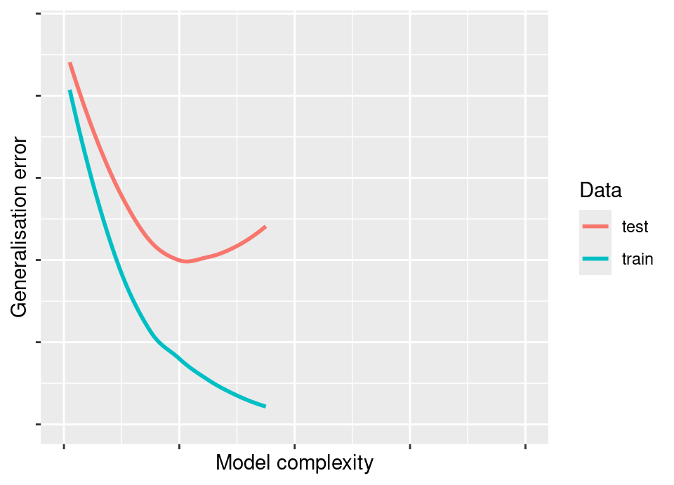
At the same time, we witness the hazard of using the training error, because this will typically appear to continue to fall well past the point at which we have good generalisation properties!

In the preliminary material, you broke down the reducible error into specifically a squared bias and a variance component and in the squared loss case these correspond to approximation and estimation errors. You also computed the total error as you varied the complexity of the model and will have observed this classic curve which falls then rises in the test error.

However, a string of very recent recent research results have demonstrated the existance of a so-called double descent phenomenon. There are many highly flexible models in which the following rather surprising behaviour has been observed:

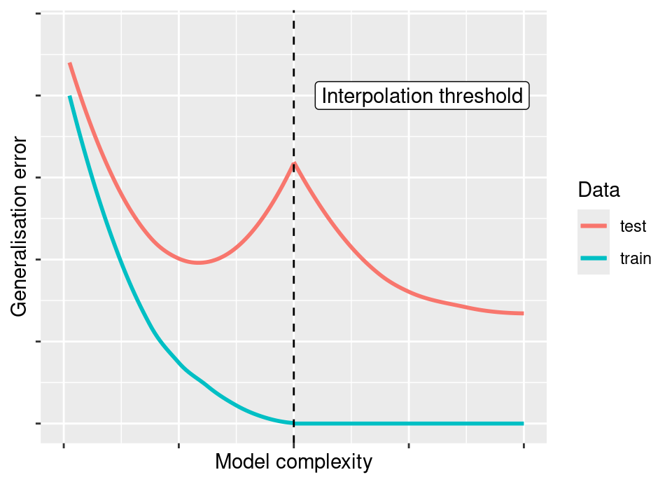
The vertical dashed line represents the “interpolation threshold”, where the complexity of the model has become sufficiently high that for the particular dataset under consideration the model perfectly interpolates all observations leading to zero training/apparent error. However, the surprising behaviour is that in some circumstances if one continues to increase model complexity we observe a second descent in the test error, it often being seen to drop lower than in the initial non-interpolating regime.

This topic is still not fully understood, being a comparatively recent development. It was first observed in large scale deep neural networks (Neyshabur et al., 2015; Zhang et al., 2017) and an accessible overview to gain some insight is Belkin et al. (2019).

3.6 Expected error and consistency

As stressed in the last section, the generalisation error relates to a fixed, fitted, model. Of course, these models are in fact fitted to data we observe which are random realisations of some unknown true generating measure, \(\pi_{XY}\). We can consider therefore, the expected error, accounting for the random nature of the model fit across hypothetical future realisations of datasets of the same size.

Let us define \(D_n := \left( (X_1, Y_1), \dots, (X_n, Y_n) \right)\) to be the random variable denoting a sample of \(n\) observations, whose joint distribution is \(\pi_{XY}^n := \underbrace{\pi_{XY} \times \dots \times \pi_{XY}}_{n \text{ times}}\), the product measure⁵ representing the law of an iid sample of data of size \(n\) from \(\pi_{XY}\). In other words, \(\mathcal{D}_n\) is a realisation of the random variable \(D_n\). To defer complex notation as long as possible we had not shown conditioning on the data hereinbefore, but we now need to make clear the data dependence of \(\hat{f}\) hereinafter with appropriate conditioning.

Definition 3.6 (expected (prediction) error) The expected error of a learning algorithm which learns \(\hat{f} \in \mathcal{F}\) given data sample \(D_n \sim \pi_{XY}^n\) is, \[\bar{\mathcal{E}}_n := \mathbb{E}_{D_n}\left[ \mathcal{E}(\hat{f}) \right] = \mathbb{E}_{D_n}\left[ \mathbb{E}_{XY}\left[ \mathcal{L}(Y, g_{\hat{f}}(X \given D_n)) \right] \right]\] Sometimes rather than an aggregate expected error we are more interested in the expected prediction error of a learning algorithm at a given predictor value \(X=\vec{x}\), \[\bar{\mathcal{E}}_n(\vec{x}) := \mathbb{E}_{D_n}\left[ \mathbb{E}_{Y \given X=\vec{x}}\left[ \mathcal{L}(Y, g_{\hat{f}}(X \given D_n)) \right] \right]\] where now the inner expectation is conditioned on the predictor.

This leads to the concept of consistency⁶.

Definition 3.7 (consistency) A learning algorithm is said to be consistent for \(\pi_{XY}\) if it is asymptotically Bayes error efficient. That is, if the expected error converges to the Bayes error in the limit as the sample size grows, \[\mathbb{E}_{D_n}\left[ \mathbb{E}_{XY}\left[ \mathcal{L}(Y, g_{\hat{f}}(X \given D_n)) \right] \right] \to \mathcal{E}^\star \text{ as } n \to \infty\] A learning algorithm is universally consistent if it is consistent for all data generating measures \(\pi_{XY}\).

Note, the above is a distinct definition from statistical consistency!

Note that finding a universally consistent learning algorithm would appear to be the nirvana of machine learning: this would be a method which can get arbitrarily close to the Bayes optimal error rate for any problem. In particular, this means it has zero approximation error and an estimation error which tends to zero as available data increases (see §3.5.1). However, the devil always being in the detail, this universal consistency tells us nothing about quite how much data is necessary to get within some desired tolerance of that Bayes error rate. As we shall see, universally consistent learning methods do exist but can be data hungry because the very flexibility which provides universality demands a lot of data to train, whilst approaches which lack universality can converge faster if you have chosen the correct model class.

We now have multiple notions of error, so it may be instructive to note the relationship between them:

*Relationship between types of error*
	Fixed inputs	Random inputs
Fixed training set	\(\text{Err}(\cdot)\)	\(\mathcal{E}(\cdot)\)
Random training set	\(\star\)	\(\bar{\mathcal{E}}_n(\cdot)\)

The columns indicate whether we are considering prediction at fixed inputs (the location of \(\mat{X}\) in the training data), or random inputs (draws from \(\pi_X\)). The columns indicate whether we are thinking about the error made by the particular model we have fitted to a particular training data set (the particular \(\mathcal{D}\) we have observed) or the error made by the learning method across hypothetical future datasets (drawn repeatedly from \(\pi_{XY}^n\) to train). Note, we do not consider setting \(\star\) here (see Rosset and Tibshirani, 2020 if you are interested in this).

All these errors may be interesting in different contexts. Just one example for each:

\(\text{Err}(\cdot)\) is the classic setting often studied in a standard statistical modelling settings, where I have perhaps carefully designed the collection of data.
If I am conducting an application and wish to deploy a model for real world use, I am most likely interested in \(\mathcal{E}(\cdot)\) because this gives me information about future performance for my given fixed model.
If I am developing new methodology or understanding the behaviour of existing methodology, I am most likely interested in \(\bar{\mathcal{E}}_n(\cdot)\) because this gives me information about future performance under hypothetical repeated model fits and prediction from a certain population.

In particular in thinking about these and the methods deployed to evaluate the errors, care may be required in possible hidden assumptions about my data being observational in nature and therefore the distribution of \(\mat{X}\) reflective of \(\pi_X\), rather than designed.

3.6.1 More error decomposition

It can be instructive to think about decomposition of the expected error just as we considered decomposition of the generalisation error in §3.5.1. However, to make more progress we must consider a concrete modelling setup and loss function.

Example 3.8 (bias-variance decomposition of least squares) Consider again the concrete setting of a true data generating process that matches the regression setting in §3.2 (ie additive independent zero-mean error), where we aim to minimise the squared loss. Then, the expected error can be decomposed further. We start by invoking the generalisation error decomposition proved in Example 3.7 for the inner expectation: \[\mathbb{E}_{D_n} \mathbb{E}_{XY}\left[\left( Y - \hat{f}(X) \right)^2\right] = \mathbb{E}_{D_n} \mathbb{E}_{XY}\left[\left( f(X) - \hat{f}(X) \right)^2\right] + \mathbb{E}_{D_n} \mathrm{Var}_{XY}(\varepsilon)\] Of course, the variance in this expression is constant with respect to the training data so the outer expectation can be dropped from the second term, and we can focus on further decomposing the first term: \[\begin{align*} &\mathbb{E}_{D_n} \mathbb{E}_{XY}\left[\left( f(X) - \hat{f}(X) \right)^2\right] \\ &\quad= \underbrace{\mathbb{E}_{XY} \mathbb{E}_{D_n}}_{\text{Fubini-Tonelli Theorem}}\left[\left( f(X) - \hat{f}(X) \right)^2\right] \\ &\quad= \mathbb{E}_{XY} \mathbb{E}_{D_n}\left[\left( \left( f(X) - \mathbb{E}_{D_n} \hat{f}(X) \right) + \left( \mathbb{E}_{D_n} \hat{f}(X) - \hat{f}(X) \right) \right)^2\right] \quad \text{just }\pm\text{ same term} \\ &\quad= \mathbb{E}_{XY} \mathbb{E}_{D_n}\left[ \left( f(X) - \mathbb{E}_{D_n} \hat{f}(X) \right)^2 + \left( \mathbb{E}_{D_n} \hat{f}(X) - \hat{f}(X) \right)^2 \right. \\ &\quad\phantom{= \mathbb{E}_{XY} \mathbb{E}_{D_n}} \left. \vphantom{\left( f(X) - \mathbb{E}_{D_n} \hat{f}(X) \right)^2 + \left( \mathbb{E}_{D_n} \hat{f}(X) - \hat{f}(X) \right)^2} \quad+ 2 \left( f(X) - \mathbb{E}_{D_n} \hat{f}(X) \right) \left( \mathbb{E}_{D_n} \hat{f}(X) - \hat{f}(X) \right) \right] \end{align*}\] The outer expectations will pass to the three terms and we note that for the final term: \[\begin{align*} &\mathbb{E}_{XY} \mathbb{E}_{D_n}\left[ \underbrace{2 \left( f(X) - \mathbb{E}_{D_n} \hat{f}(X) \right)}_{\text{constant wrt training data}} \left( \mathbb{E}_{D_n} \hat{f}(X) - \hat{f}(X) \right) \right] \\ &\quad= 2 \mathbb{E}_{XY}\left[ \left( f(X) - \mathbb{E}_{D_n} \hat{f}(X) \right) \underbrace{\mathbb{E}_{D_n}\left[ \mathbb{E}_{D_n} \hat{f}(X) - \hat{f}(X) \right]}_{= \mathbb{E}_{D_n} \hat{f}(X) - \mathbb{E}_{D_n} \hat{f}(X) = 0} \right] \\ &\quad=0 \end{align*}\] Therefore, in full, for squared loss: \[\begin{align*} \bar{\mathcal{E}}_n &= \mathbb{E}_{XY} \mathbb{E}_{D_n}\left[ \left( f(X) - \mathbb{E}_{D_n} \hat{f}(X) \right)^2 \right] & \text{squared bias of model} \\ &\quad+ \mathbb{E}_{XY} \mathbb{E}_{D_n}\left[ \left( \mathbb{E}_{D_n} \hat{f}(X) - \hat{f}(X) \right)^2 \right] & = \mathbb{E}_{XY}\mathrm{Var}_{D_n}\hat{f}(X) \text{ variance of model fit} \\ &\quad+ \mathrm{Var}_{XY}(\varepsilon) & \text{irreducible error} \end{align*}\] You may have encountered a slightly simpler form of this which applied to the fixed inputs case (see end problem setting)

The bias-variance decomposition in Example 3.8 is central to understanding the trade-offs involved in fitting machine learning models and directly leads to the kinds of performance curves shown in §3.5.2.

The situation is substantially more complicated to analyse in terms of bias and variance with other loss functions. See for example Friedman (1997) for a discussion of 0-1 loss in this context.

3.6.2 Expected error learning curves

Another natural avenue of exploration from the expected error would lead us to consider the dependence of the learning method’s performance on dataset size, both to understand the learning efficiency in each context and to predict how beneficial larger training data sets might be. Questions of this variety can be addressed via both theoretical and empirical examination of the learning curve: that is, the plot of \(\bar{\mathcal{E}}_n\) (or an empirical estimate of it) against \(n\) (Viering and Loog, 2021). A well-behaved learning curve will be monotonically decreasing, \(\bar{\mathcal{E}}_n \ge \bar{\mathcal{E}}_{n+1}\), and one can compute empirical estimators of the learning curve to compare learning rates in specific applications.

There is an extension of the above, called the problem-average learning curve, where a further expectation is taken over the distribution of problems, that is over varying \(\pi_{XY}\) (most naturally thought of in a Bayesian manner).

For an example of code applying learning curves, see §7.1.5.

3.7 Model fitting

Thus far we have assumed there exists some means of selecting \(\hat{f}\) without explicitly discussing how. Of course, given a full probabilistic model, we should proceed (as good statisticians!) to conduct a standard likelihood or full Bayesian analysis to fit the model \(\hat{f}\), and identify the best predictor \(g_{\hat{f}}\) using the Bayes predictor to guide us, per the discussion in the previous section. However, many machine learning methods, which we will study in due course, lack a formal probabilistic model and are fitted by directly considering the empirical generalisation error under the target loss of interest.

Therefore, we have broadly three settings: (i) a full probabilistic model; (ii) a parametric family for \(f\) without an explicit probabilistic model; and (iii) local methods to directly construct non-parametric empirical estimates. We assume anyone taking this course is already intimately familiar with (i) and also refer to the APTS Statistical Modelling module (Ogden et al., 2021). Therefore, we cover (ii)+(iii) first, then comment on the importance of (i) afterwards in §3.7.3 (a point doubtless obvious to the audience of this course!)

3.7.1 Parametric families

In this setting we specify a model family (or hypothesis space) \(\mathcal{F}\) according to some parametric family, but without a full probabilistic specification. Arguably the simplest example is linear regression without the assumption of Gaussian errors, so that \(\mathcal{F} = \{ f(\vec{x}) = \vec{x}^T \vecg{\beta} : \vecg{\beta} \in \mathbb{R}^d \}\).

Absent any probabilistic specification for the errors, such models are usually fitted by performing so-called Empirical Risk Minimisation (ERM) directly against a target loss of subject-matter interest. Perhaps a little surprisingly to a statistician, it unfortunately not unheard of for machine learners to use ERM even where there is a natural probabilistic structure, but here we would advocate standard statistical methods in that situation.

Definition 3.8 (empirical risk minimisation) Let \(\mathcal{F}\) be a model family (or hypothesis space) parameterised by \(\theta \in \Theta\). Assume we have a dataset \(\mathcal{D} = \left( (\vec{x}_1, y_1), \dots, (\vec{x}_n, y_n) \right)\), where \((\vec{x}_i, y_i) \overset{iid}{\sim} \pi_{XY}\). Then we fit a model \(\hat{f}\in\mathcal{F}\) to \(\mathcal{D}\) using empirical risk minimisation of a loss function of interest \(\mathcal{L}(\cdot,\cdot)\) as \[\hat{f}(\cdot) = f(\cdot \given \hat{\theta}) \text{ where } \hat{\theta} = \arg\min_{\theta \in \Theta} \sum_{(x,y)\in\mathcal{D}} \mathcal{L}(y, f(x \given \theta))\] if this minimum exists.

In the parametric context, the parameter \(\theta\) defines the function space, \[\mathcal{F} = \{ f(\cdot \given \theta) : \theta \in \Theta \}\]

ERM is, therefore, essentially an optimisation problem. Aside from some very special cases which posses a closed form solution (eg least squares linear regression), this means that we usually deploy some variant of gradient descent to find the minimising parameter. Note that if one performs ERM using our ultimate target loss of interest, it is then by definition the case that simply \(g_{\hat{f}} = \hat{f}\).

3.7.2 Non-parametric local methods

There are a collection of non-parametric approaches which seek to directly construct a purely empirical estimate of the Bayes predictor directly, without any explicit ‘model fitting’ step.

Arguably the simplest example of this is the \(k\)-nearest neighbours algorithm, which we will cover in more detail in §4.1. Imagining that the target loss function of interest is squared loss, then we know that the optimal Bayes predictor is \(g^\star(\vec{x}) = \mathbb{E}[Y \given X = \vec{x}]\). The \(k\)-nearest neighbour algorithm therefore directly empirically estimates \(\mathbb{E}[Y \given X = \vec{x}]\) by selecting the \(k \in \mathbb{N}^+\) observations in the dataset \(\mathcal{D}\) which are ‘nearest’ (by some metric, \(d : \mathcal{X} \times \mathcal{X} \to [0,\infty)\)) to \(\vec{x}\), then empirically estimating the required expectation. That is, if we reorder the data \(\mathcal{D} = \left( (\vec{x}_1, y_1), \dots, (\vec{x}_n, y_n) \right)\) by increasing values of \(d(\vec{x}_i, \vec{x})\) and define this ordering by \(\left( (\vec{x}_{(1)}, y_{(1)}), \dots, (\vec{x}_{(n)}, y_{(n)}) \right)\), then \[\hat{f}(\vec{x}) := \frac{1}{k} \sum_{i = 1}^k y_{(i)}\]

Local methods have the benefit of being both conceptually simple and easy to implement, but there are many drawbacks including computational, scaling in dimension and overfitting risk. These will be discussed further in Chapter 4.

3.7.3 Statistical methods

The thrust of this section is likely self-evident to the audience of this course, but bears mention for completeness. Note that in the presence of a plausible probabilistic model (which has had assumptions carefully checked) we should favour leveraging our statistical knowledge, rather than blindly performing ERM to fit said model: it is not automatic that model fitting against a target loss gives the best predictive performance against that loss. Unsurprisingly, if the assumptions of a full probabilistic model are approximately satisfied, then use of full likelihood or Bayesian methods will usually result in a better model fit and consequently better predictive performance.

Consider the most extreme trivial setting by way of counter-example against blindly using ERM in the presence of a probabilistic model. Let us predict a response \(Y\) using no features, where interest is in achieving the lowest mean absolute generalisation error. Assume that Normality appears satisfied so that we have a probabilistic formulation. The median and mean are the same, \(\mu\), for a Normal distribution, but we know that the sample mean has variance \(\frac{\sigma^2}{n}\), whilst the sample median has variance \(\frac{\pi \sigma^2}{2n}\). Therefore, we would still prefer to estimate \(\mu\) via the likelihood (equivalent to minimising mean square error) when ‘fitting’ this model, despite the stated aim of achieving lowest mean absolute generalisation error because the variance of the sample mean is smaller than that of the sample median. Of course, if Normality is violated here, the situation can change dramatically: for example, with t-distributed data, MSE would outperform when there are 5 or more degrees of freedom, and one would be better directly optimising MAE otherwise.

The above example is not the only case and this intuition carries over to the simple linear model setting too, as empirically illustrated in the following R code, which examines minimising MAE in Example 3.3. We observe that in this case, fitting by minimising MSE tends to achieve lower generalisation error for both MSE and MAE than fitting by directly minimising MAE, precisely because we are accounting for probabilistic structure that is indeed present.

# Set the "true" values for beta
beta <- c(1.2, -0.35)

# Monte Carlo estimate of the MSE and MAE generalisation error that arises from
# using MSE or MAE as the model fitting loss
msehattst.msefit <- c()
maehattst.msefit <- c()
msehattst.maefit <- c()
maehattst.maefit <- c()
for(i in 1:5000) {
  # Sample 20 new training observations from \pi_{XY}
  X <- matrix(runif(20*2), ncol = 2)
  y <- X%*%beta + rnorm(nrow(X))

  # Compute \hat{\beta} targeting MSE for model fit
  betahat.mse <- solve(crossprod(X))%*%t(X)%*%y
  # Compute \hat{\beta} targeting MAE for model fit
  # Using a numerical optimiser, so check convergence and rerun from a different random location
  # if convergence fails
  while((opt <- optim(runif(2, -2, 2), function(b) { mean(abs(y-X%*%b)) }))$convergence != 0) { }
  betahat.mae <- matrix(opt$par, ncol = 1)

  # Generate an (unrealistically) large testing set
  X <- matrix(runif(20*2), ncol = 2)
  y <- X%*%beta + rnorm(nrow(X))
  msehattst.msefit <- c(msehattst.msefit, mean((y-X%*%betahat.mse)^2))
  maehattst.msefit <- c(maehattst.msefit, mean(abs(y-X%*%betahat.mse)))
  msehattst.maefit <- c(msehattst.maefit, mean((y-X%*%betahat.mae)^2))
  maehattst.maefit <- c(maehattst.maefit, mean(abs(y-X%*%betahat.mae)))
}

# Result
table("MSE fit better for MAE generalisation error" = (maehattst.msefit < maehattst.maefit))
cat(paste0("MSE better in ", mean(maehattst.msefit < maehattst.maefit)*100, "% of the runs"))

table("MSE fit better for MSE generalisation error" = (msehattst.msefit < msehattst.maefit))
cat(paste0("MSE better in ", mean(msehattst.msefit < msehattst.maefit)*100, "% of the runs"))

Further cautionary examples are quite easy to construct, which show that a full likelihood model fit gives better predictive performance than directly minimising MSE/MAE/etc. As indicated, this should come as no surprise to a seasoned statistician, but bears emphasising given much non-statistical material written on machine learning ignores this point.

3.7.4 Regularisation

In order to avoid overfitting, or in the overparameterised regime (due either to small data or seeking a second descent in the risk curve), we may need to apply regularisation to our overall loss. In this setting, rather than minimising only the loss, we would minimise:

\[\arg\min_{\theta \in \Theta} \sum_{(x,y)\in\mathcal{D}} \mathcal{L}(y, f(x \given \theta)) + \lambda C(\theta)\]

where \(C(\theta)\) measures the model complexity and \(\lambda\) controls the extent of regularisation. For example, in ridge regression, \(C(\theta) = \| \theta \|_2^2\), or for lasso regression, \(C(\theta) = \| \theta \|_1\)

We simply note that regularisation can be used in the machine learning framework via this generic construction, but omit details since this was the topic of the High-dimensional Statistics APTS course (Yu, 2021).

3.8 Proper scoring rules

Not all losses are created equally. In particular, if we are using a method which can provide a probabilistic forecast (eg simple linear regression with Normal errors; or probabilistic classifiers like logistic regression; etc), then we should be especially concerned with evaluating not only whether a “best guess” point estimate is good, but in fact whether our whole probabilistic forecast is good. This is called calibration, and we know from the statistics literature (Gneiting and Raftery, 2007) that losses which satisfy the conditions for a proper scoring rule will provide probabilistic calibration (see §7.1.4 for a discussion of assessing calibration in applications).

The following definition is adapted to the notation and context of this Chapter:

Definition 3.9 ((strictly) proper scoring rule) Let \(\mathcal{P}\) be the space of probability distributions on \(\mathcal{Y}\). Then a scoring rule is a function \[S: \mathcal{P} \times \mathcal{Y} \to \mathbb{R}\] which provides a numerical value to any probabilistic prediction \(P \in \mathcal{P}\) and associated outcome \(y \in \mathcal{Y}\).

A scoring rule is said to be a proper scoring rule if \[\mathbb{E}_{Y \given X} S(\pi_{Y \given X},Y) \ge \mathbb{E}_{Y \given X} S(P,Y) \ \forall\,P\in\mathcal{P}\] The rule is said to be strictly proper when equality occurs if and only if \(P \equiv \pi_{Y \given X}\).

A strictly proper scoring rule ensures that there is no benefit to producing any probabilistic forecast which is not exactly calibrated with the truth. If a scoring rule is not strictly proper (or worse, is improper) then the model could achieve a maximal score even though the probabilistic forecast is mis-calibrated.

The following plot (based on an example in Štrumbelj, 2018) shows this for some classification losses. The first row of the plot gives 5 different models for the response of a 3 label classification problem (assume no features). Model 1 is the ‘true’ model and defines \(\pi_{Y}\). The second row of the plot shows the value of the generalisation error computed using 3 different losses for each model.

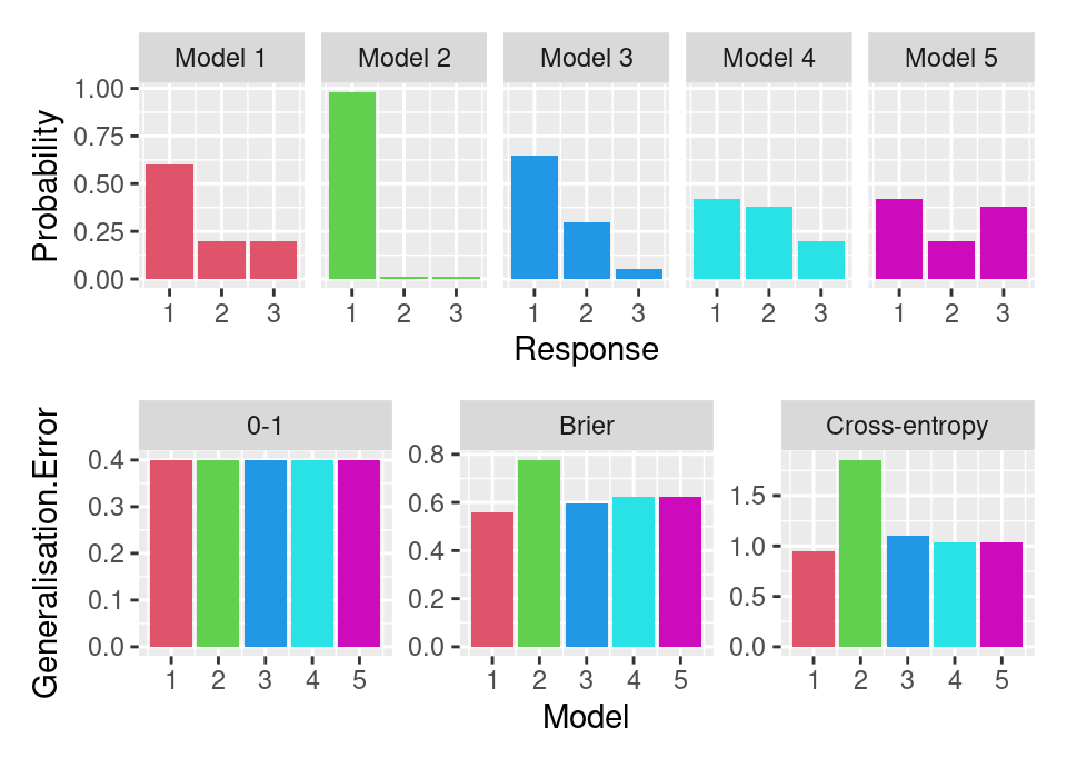
The Brier and cross-entropy, being strictly proper scoring rules, correctly assign model 1 the smallest generalisation error. However, 0-1 loss which is not strictly proper (only proper), actually assigns all models the same generalisation error! Consequently, 0-1 loss fails to correctly identify the calibrated true model. Note that Brier and cross-entropy do none-the-less disagree on the ordering of the remaining models.

3.9 Limitations

There can be few who do not know the precept due to George Box, by which statisticians work. It is often abbreviated and appeared in multiple places in his book:

“Remember that all models are wrong; the practical question is how wrong do they have to be to not be useful.”

— Box and Draper (1987), pp.74

“[…] all models are approximations. Essentially, all models are wrong, but some are useful. However, the approximate nature of the model must always be borne in mind.”

— Box and Draper (1987), pp.424

This is every bit as true in machine learning, tempting though it may be to think that the reduction of assumptions (compared to standard statistical modelling) might lead to some universally best method. Indeed, the fact we have universally consistent (Definition 3.7) methods might, at a cursory glance, suggestively nod in that direction. However, we live in a world of finite data and it is possible to prove there is no universally best method for a finite fixed sample size \(n\). Indeed, small sample size settings need to be especially cognoscent of how fast different methods learn: the more flexible approaches can be empirically observed to require large amounts of data to fit well (van der Ploeg et al., 2014).

Consider the case of binary classification (see Devroye et al. (1996), Theorem 7.1):

Theorem 3.1 Let \(\varepsilon>0\) be an arbitrarily small real value. For any integer \(n\) and classification rule \(g_n\), there exists a distribution \(\pi_{XY}\) (for \(\mathcal{Y}\) binary) with Bayes error zero, \(\mathcal{E}^\star = 0\), such that \[\bar{\mathcal{E}}_n = \mathbb{E}_{D_n}\left[ \mathbb{E}_{XY}\left[ \mathcal{L}(Y, g_n(X \given D_n)) \right] \right] \ge \frac{1}{2} - \varepsilon\] when \(\mathcal{L}\) is 0-1 loss.

That is, for any sample size \(n\) there exists a distribution \(\pi_{XY}\) for which the learning method performs arbitrarily badly.

This is one of many so-called “no free lunch theorems” (Wolpert, 1996) in machine learning which essentially show that given any learning methodology there exists some data distribution upon which it will perform arbitrarily badly.

3.10 Further reading

This short course aims to balance a brief introduction to theory, methodology, and application in statistical machine learning, so we will not go further into the theory here. However, a highly recommended text (currently being drafted at the time of writing) is Bach (2021) for full development from a learning theory side. A more theoretical treatment would be in Mohri et al. (2018), which develops the topic within the Probably Approximately Correct (PAC) learning theory framework (sadly, time did not permit introducing this here). There are also older text books with a learning theoretic slant which are interesting reads, including Devroye et al. (1996) and Vapnik (1998).

This Chapter has introduced some of the elementary learning theory that underpins the supervised machine learning problem, which provides a mental model for understanding the methodology and practical application of these techniques. We proceed next to consider some machine learning methods.

References

Bach, F. (2021). Learning Theory from First Principles, Draft. ed. URL https://www.di.ens.fr/~fbach/ltfp_book.pdf

Belkin, M., Hsu, D., Ma, S., Mandal, S. (2019). Reconciling modern machine-learning practice and the classical bias–variance trade-off. Proceedings of the National Academy of Sciences 116(32), 15849–15854. DOI: 10.1073/pnas.1903070116

Bernardo, J.M., Smith, A.F.M. (1994). Bayesian Theory, 1st ed, Wiley Series in Probability and Statistics. Wiley. ISBN: 978-0471494645

Box, G.E.P., Draper, N.R. (1987). Empirical model-building and response surfaces, 1st ed, Wiley series in probability and statistics. Wiley. ISBN: 978-0471810339

Breiman, L., Spector, P. (1992). Submodel selection and evaluation in regression. The \(X\)-random case. International Statistical Review 60(3), 291–319. DOI: 10.2307/1403680

DeGroot, M.H., Schervish, M.J. (2012). Probability and Statistics, 4th ed. Pearson. ISBN: 978-0321500465

Devroye, L., Györfi, L., Lugosi, G. (1996). A Probabilistic Theory of Pattern Recognition, 1st ed. Springer. ISBN: 978-0387946184

Friedman, J.H. (1997). On bias, variance, 0/1-loss, and the curse-of-dimensionality. Data Mining and Knowledge Discovery 1, 55–77. DOI: 10.1023/A:1009778005914

Gneiting, T., Raftery, A.E. (2007). Strictly proper scoring rules, prediction, and estimation. Journal of the American Statistical Association 102(477), 359–378. DOI: 10.1198/016214506000001437

Hastie, T., Tibshirani, R., Friedman, J. (2009). The Elements of Statistical Learning, 2nd ed, Springer Series in Statistics. Springer. URL https://web.stanford.edu/~hastie/ElemStatLearn/printings/ESLII_print12_toc.pdf, ISBN: 978-0387848570

James, G., Witten, D., Hastie, T., Tibshirani, R. (2013). An Introduction to Statistical Learning, 1st ed, Springer Texts in Statistics. Springer. URL https://www.statlearning.com/s/ISLR-Seventh-Printing.pdf, ISBN: 978-1461471370

Mohri, M., Rostamizadeh, A., Talwalkar, A. (2018). Foundations of Machine Learning, 2nd ed. MIT Press. URL https://www.dropbox.com/s/7voitv0vt24c88s/10290.pdf?dl=1, ISBN: 978-0262039406

Neyshabur, B., Tomioka, R., Srebro, N. (2015). In search of the real inductive bias: On the role of implicit regularization in deep learning, in: Proceedings of the Third International Conference on Learning Representations. URL https://arxiv.org/abs/1412.6614

Ng, A.Y., Jordan, M.I. (2001). On discriminative vs. Generative classifiers: A comparison of logistic regression and naive bayes, in: Proceedings of the 14th International Conference on Neural Information Processing Systems. pp. 841–848. URL http://papers.nips.cc/paper/2020-on-discriminative-vs-generative-classifiers-a-comparison-of-logistic-regression-and-naive-bayes.pdf

Ogden, H.E., Davison, A.C., Forster, J.J., Woods, D.C., Overstall, A.M. (2021). APTS: Statistical Modelling Notes. URL https://warwick.ac.uk/fac/sci/statistics/apts/students/resources/statmod-notes.pdf

Robert, C.P. (2007). The Bayesian Choice, 2nd ed, Springer Texts in Statistics. Springer. ISBN: 978-0387715988

Rosset, S., Tibshirani, R.J. (2020). From fixed-x to random-x regression: Bias-variance decompositions, covariance penalties, and prediction error estimation. Journal of the American Statistical Association 115(529), 138–151. DOI: 10.1080/01621459.2018.1424632

Shaw, S.C., Rougier, J.C. (2020). APTS: Statistical Inference Notes. URL https://warwick.ac.uk/fac/sci/statistics/apts/students/resources/lecturenotes.pdf

Štrumbelj, E. (2018). Predictive model evaluation. Course Notes. URL https://file.biolab.si/textbooks/ml1/model-evaluation.pdf

van der Ploeg, T., Austin, P.C., Steyerberg, E.W. (2014). Modern modelling techniques are data hungry: A simulation study for predicting dichotomous endpoints. BMC Medical Research Methodology 14(137). DOI: 10.1186/1471-2288-14-137

Vapnik, V.N. (1998). The Nature of Statistical Learning Theory, 2nd ed. Springer. ISBN: 978-0387987804

Viering, T., Loog, M. (2021). The shape of learning curves: A review. arXiv (2103.10948). URL https://arxiv.org/abs/2103.10948

Wang, J., Shen, X. (2006). Estimation of generalization error: Random and fixed inputs. Statistica Sinica 16(2), 569–588. URL http://www3.stat.sinica.edu.tw/statistica/J16N2/J16N213/J16N213.html

Wolpert, D.H. (1996). The lack of a priori distinctions between learning algorithms. Neural Computation 8, 1341–1390. DOI: 10.1162/neco.1996.8.7.1341

Yu, Y. (2021). APTS: High-dimensional Statistics Notes. URL https://warwick.ac.uk/fac/sci/statistics/apts/students/resources/hdsnotes.pdf

Zhang, C., Bengio, S., Hardt, M., Recht, B., Vinyals, O. (2017). Understanding deep learning requires rethinking generalization, in: Proceedings of the Fifth International Conference on Learning Representations. URL https://arxiv.org/abs/1611.03530

You will encounter some texts which assign \(\pm 1\) rather than \(\{0,1\}\) as the response in binary classification problems.↩︎
Time series data being a notable exception, among others.↩︎
Be sure not to confuse this with the problem of handling uncertainty in the predictors (ie that they may suffer noise or be imprecisely observed) … that is a well studied but entirely different problem. Here we simply mean that the model will be used to make predictions at unknown future values of the features \(\vec{x}\).↩︎
This is loose notation: in theory an identical (in value) observation can of course be in \(\mathcal{D'}\) and \(\mathcal{D}\) as long as they arose as iid samples from \(\pi_{XY}\).↩︎
In the standard way, that is the product of measures \(\pi_1\) and \(\pi_2\) is defined to be \((\pi_2 \times \pi_2)(A_1 \times A_2) = \pi_1(A_1) \pi_2(A_2)\) for measurable subsets \(A_1\) and \(A_2\).↩︎
There is another notion of consistency which starts from a different perspective, that of so-called Probably Approximately Correct (PAC) learning. It would be too great a diversion to present this here, but the textbook Mohri et al. (2018) takes this approach and can be consulted by the curious reader.↩︎