Chapter 7 Model Assessment and Combination
We turn our attention from theory and methodology towards highlighting some practical concerns around assessing model performance. This discussion will be primarily in the classification context where there can be subtlety in evaluation. We also examine some common strategies for model combination, since there is no universally dominant machine learning algorithm, we often find improved performance from using a suite of methods in concert.
7.1 Assessment of classification models
We will root this discussion in the binary classification case for consistency and ease of understanding, though some of the observations apply more generally.
The naïve assessment of a classification model relies on the accuracy, this being simply 1 minus the misclassification rate (ie 1 minus 0-1 loss). One may find, especially when working on applied problems with non-experts, this is the figure most often requested.
Casting our minds back to §3.5, we know that we should report the Bayes optimal predictor under 0-1 loss to therefore achieve the best accuracy possible given our model:
\[g^\star(\vec{x}) = \arg\max_{j \in \{1,\dots,g\}} f_j(\vec{x})\]
That is, for best accuracy we should select whichever label has the highest probability of being observed according to the model. However, it usually requires very little probing of an applied problem to discover it is actually rather rare in practice that simple accuracy is really the quantity of interest.
Indeed, an unhealthy obsession with accuracy can often lead to potentially dubious procedures which attempt to “fix” problems that in many cases do not need to be fixed. A classic example of this is imbalanced data, where the proportion of each binary response observed in the training dataset is far from being 50-50. It is then not unusual to see over or under-sampling approaches employed in an attempt to rescue this inappropriate metric, when in many cases all that is required is good probabilistic estimation, understanding of the population prevalence of the outcomes, and correct specification of the loss (also note, if sampling was originally random and under/over-sampling is used, we then break the assumption that samples are from \(\pi_{XY}\) and furthermore lose calibration!)
Even when applied classification problems ultimately need to provide a predicted label (though hopefully our statistical predilection compels us to also report probabilities alongside), fitting a carefully calibrated probabilistic output and then selecting a problem-specific classification cutoff is far preferable to unthinking application of a Bayes optimal choice for what is often fundamentally the wrong loss.
7.1.1 Baseline models
Before discussing these matters, we highlight a common omission when reporting the performance of machine learning models: failure to include a simple baseline model. What do we mean by this? At the simplest level, this is the model which just predicts the most common class in the training data, irrespective of the features:
\[\hat{f}_j(\vec{x}) = \begin{cases} 1 & \text{if } \sum_{i \in \mathcal{T}_r} \bbone\{ y_i = j \} > \sum_{i \in \mathcal{T}_r} \bbone\{ y_i = k \} \ \forall\, k \\ 0 & \text{otherwise} \end{cases}\]
When looking at accuracy in an imbalanced dataset, this is a particularly important baseline to include, since in extreme cases high accuracy will be achieved simply due to the imbalance. Another baseline model that is wise to include is a standard un-regularised logistic regression.
It is always good practice to include the baseline model(s) in all your performance evaluations so that you are fully informed about how much (if any) benefit your sophisticated machine learning model is gaining. The reason for this is that you might be surprised how often a baseline model like logistic regression is entirely adequate! (Christodoulou et al., 2019) If logistic regression is close enough to the performance of a far more complex method, it would be prudent to use the simpler model.
7.1.2 Cut-off selection
The Bayes optimal choice under 0-1 loss corresponds to having a cutoff of 0.5 for reporting a predicted “1”:
\[g^\star(\vec{x}) = \arg\max_{j \in \{0,1\}} f_j(\vec{x}) = \begin{cases} 0 & \text{if } f_1(\vec{x}) < 0.5 \\ 1 & \text{if } f_1(\vec{x}) \ge 0.5 \end{cases}\]
However, if 0-1 loss is not the actual true representation of our loss then this is not necessarily Bayes optimal (the point is, by now, becoming laboured hopefully!). We can actually choose any cutoff value \(\alpha \in [0,1]\) we wish:
\[g_{\hat{f}}(\vec{x}) = \begin{cases} 0 & \text{if } \hat{f}_1(\vec{x}) < \alpha \\ 1 & \text{if } \hat{f}_1(\vec{x}) \ge \alpha \end{cases}\]
Recall the careful distinction drawn early in the course between a loss used for model fitting and a loss used to ultimately make a decision (this should not feel strange to us as statisticians, where we are comfortable with fitting a model using likelihood/Bayesian methods and then specify a loss for decision making). At the very least, we should ensure we are using a proper scoring rule (§3.8) to ensure we get good probabilistic calibration and then specify a target loss of concern for decision making.
Informally, there are a variety of important measures which can be helpful to analyse in applied classification problems, often being of interest for informal reasoning about the problem (there will be a corresponding implied loss that is effectively minimised by any selection on these scales). Many of these will likely be familiar already, so we just provide a brief reminder:
- True positive (TP) rate (aka sensitivity or recall): is the conditional probability of correctly predicting 1 given true label 1.
- True negative (TN) rate (aka specificity): is the conditional probability of correctly predicting a 0 given true label 0.
- False positive (FP) rate: probability of Type I error (ie 1-specificity).
- False negative (FN) rate: probability of Type II error (ie 1-sensitivity).
- Positive predictive value (PPV) (aka precision): is the conditional probability of the true label being 1 given a prediction of 1.
- Negative predictive value (NPV): is the conditional probability of the true label being 0 given a prediction of 0.
In fact, Wikipedia has a surprisingly good table of these quantities that I am unlikely to improve upon:
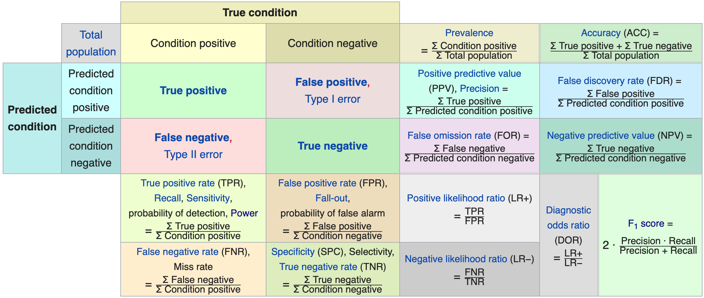
Source: Wikipedia
Crucially, each of these quantities will change as we vary the cutoff, \(\alpha\), which determines whether we predict 0 or 1. In most applications we may have a clear requirement to favour low error rates for a particular response, for example:
- Medical screening, with 1=diseased: here we will be especially concerned that we identify diseased patients, that is, we don’t miss any true 1’s. Missing true 0’s might just involve additional testing being undertaken (which if not invasive could be acceptable).
- Bank credit scoring, with 1=loan repaid: here we will be especially concerned that we identify loans that default, that is, we don’t want to miss true 0’s, since this corresponds to loans made which are never repaid. Missing true 1’s corresponds to missed profit opportunities, but doesn’t suffer an actual loss.
Therefore, we should examine the performance of the model over a range of cutoff choices in our hold-out or cross validation set, potentially assigning asymmetric costs to understand the optimal choice. It is (somewhat) alarming how rarely these issues are carefully thought through in many applied ML settings!
A final word: it is also important to think carefully about whether TP or PPV/TN or NPV (for example) is the measure of real interest. It is not uncommon to see the TP rate discussed as though the order of conditioning was actually that of the PPV, so do ensure you are actually analysing the correct quantity for your problem. For example, in a medical setting, the TP rate will help us understand the proportion of diseased people that the screening will correctly identify, but it is not the correct quantity for individual decision making for a patient. An individual patient is more interested in the PPV, that is, what proportion of positive tested patients will actually have the disease.
Finally, although these have a conditional probabilistic interpretation, they are fundamentally measures of discriminative strength, since every individual probability is dichotomised into a ‘0’/‘1’ prediction. We may prefer to think hard about calibration at the individual prediction level.
7.1.3 ROC/AUC
We cover ROC curves and AUC primarily because of their prevalence: it is important for you to know about them. However, care is required to ensure they are appropriately used.
Indeed, the Receiver Operator Characteristic (ROC) curve is possibly the most well known visualisation of classification error rates, which traces out the path of TP-vs-FP rate as \(\alpha\) varies. That is, when \(\alpha=0\) all test observations are labelled 1, resulting in 100% TP rate and 100% FP rate, with these rates falling as \(\alpha\) increases, until \(\alpha=1\) at which point all test observations are labelled 0, resulting in 0% TP rate and 0% FP rate.
Thus, a theoretical ROC curve traces the path defined by:
\[\begin{align*} (x,y) &= (FP(\alpha), TP(\alpha)), \quad \alpha \in [0,1] \\ FP(\alpha) &= \int_\mathcal{X} \bbone\{ f(\vec{x}) \ge \alpha \} d\pi_{X \given Y = 0} \\ TP(\alpha) &= \int_\mathcal{X} \bbone\{ f(\vec{x}) \ge \alpha \} d\pi_{X \given Y = 1} \end{align*}\]Of course, we cannot plot this since we do not know \(\pi_{XY}\), but we approximate it by taking a hold-out test set of observation indices, \(\mathcal{T}_e\), then computing \(\{\hat{f}(\vec{x}_i)\}_{i\in\mathcal{T}_e}\) and empirically estimating:
\[\begin{align*} (x,y) &= (\widehat{FP}(\alpha), \widehat{TP}(\alpha)), \quad \alpha \in [0,1] \\ \widehat{FP}(\alpha) &= \frac{|\{ i : \hat{f}(\vec{x}_i) \ge \alpha \cap y_i = 0, i \in \mathcal{T}_e \}|}{|\{ i : y_i = 0, i \in \mathcal{T}_e \}|} \\ \widehat{TP}(\alpha) &= \frac{|\{ i : \hat{f}(\vec{x}_i) \ge \alpha \cap y_i = 1, i \in \mathcal{T}_e \}|}{|\{ i : y_i = 1, i \in \mathcal{T}_e \}|} \end{align*}\]This for example leads to the following plot for a small random forest fitted to the spam data in Hastie et al. (2009):
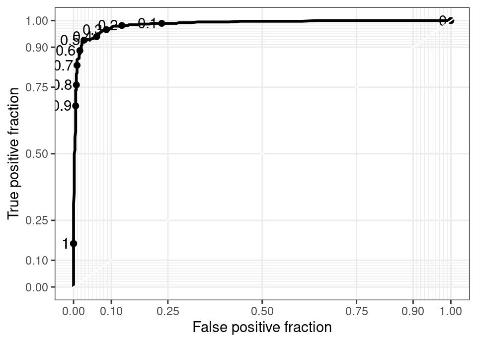
Marked on this plot by dots are the values of \(\alpha\) which give rise to that combination of TP and FP.
The following illustrates the theoretically perfect ROC curve, as well as the line that arises when the classifier performs no better than random guessing.
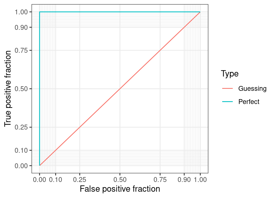
Note that any curve which falls below the \(y=x\) line (ie worse than random guess) is trivially transformed into a better than random classifier by simply acting on the opposite of the prediction. Therefore, no ROC curve should lie entirely below this line.
Given the above, one natural aggregate numerical measure of how good a ROC curve is can be given by the Area Under the Curve (AUC), which takes the empirical integral over FP giving a score \(\in [0.5,1]\) (below 0.5 indicating one should reverse the predictions).
The mathematical interpretation of the AUC is as the probability that the model ranks a randomly selected true 1 label more highly than a randomly selected true 0 label. As such, the AUC is invariant to the selected threshold. However, this can be problematic because it also doesn’t account in any way for calibration (see below), and could be a poor choice as a metric to minimize during fitting (not a proper scoring rule). In particular, it tells one very little about a particular prediction made from the model using a fixed cutoff!
Therefore, ROC and AUC require care in use. We would argue that in most settings (with exceptions) the focus should be on individual decision making and choosing the Bayes optimal decision for a well specified loss. For a given problem the ROC curve may be fundamentally conditioning on the wrong quantity: it is a visualisation conditioned on the true label, not conditioned on the prediction! That is not to say ROC curves have no use, but they should not drive a final model choice and instead may be considered more as exploratory (and, if you do applied work, you will find practitioners often ask for them!)
A possible counterpoint to this argument is if the ML model is to be deployed in “low stakes” type problems, like ad-click prediction, where an informal treatment may be adequate. However, when deploying for “high stakes” type problems, like medical prediction, a more formal contemplation of appropriate loss functions is best practice.
See Hand and Till (2001) for a proposal for how to extend the ROC and AUC to multiple label classification problems.
Computing the ROC/AUC: To plot the ROC and compute the AUC in R there are a variety of choices of package. One that produces visually appealing results is plotROC (Sachs, 2017). The following computes the AUC and plots the ROC curve for the spam data (Hastie et al., 2009) fitting a random forst and knn model for comparison.
library("randomForest")
library("e1071")
library("ggplot2")
library("plotROC")

set.seed(212)

# Load the spam data
data("spam", package = "ElemStatLearn")

# Do simple train/test 80/20 split
i <- sample(1:nrow(spam), round(nrow(spam)*0.8))
tr <- spam[i,]
te <- spam[-i,]

# Fit a small random forest (only small for compute time)
fit.rf <- randomForest(spam ~ ., tr, ntree = 200)

# Compute 7-nearest neighbour (may want to choose k with cross validation)
fit.knn <- gknn(spam ~ ., tr, k = 7)

# Gather the truth and predictive probabilities for each model
true.pred <- rbind(data.frame(model = "rf",  spam = te$spam, p = predict(fit.rf, te, type = "prob")[,"spam"]),
                   data.frame(model = "knn", spam = te$spam, p = predict(fit.knn, te, type = "prob")[,"spam"]))

# Use plotROC package to compute the ROC curve
p <- ggplot(true.pred, aes(d = as.numeric(spam)-1, m = p, colour = model)) +
  geom_roc(cutoffs.at = (0:10)/10) +
  style_roc()

# Compute the AUC and then plot
calc_auc(p)
print(p)
When you run the above, you will see that the random forest ROC curve dominates the 7-nearest neighbour across the whole range. If they crossed then we would want to think more carefully about what FP or TP rate we desired before choosing a model. We also note that the 7-nearest neighbour AUC here is 0.949 and for the random forest it is 0.986.
7.1.4 Calibration
The last two subsections discussed measures which evaluate discriminatory performance. The process of taking an individual probability (or scoring) prediction evaluating performance at a single (or spectrum) of cut-offs is essentially discarding crucial information at the individual level. Where it is possible, we may want to actually retain the observation level probabilistic forecast and ensure it is well calibrated, so that we can use them for individual decision making. Unfortunately, despite the critical importance of calibration, it is all too often overlooked in model assessment (eg in medical modelling Collins and Moons, 2012).
Informally, “well calibrated” means that the probabilistic predictions of a model exhibit good frequency properties: that is, when the model predicts ‘1’ with probability 0.7, this occurs roughly 70% of the time. This can be formalised in a few different ways, with probably the earliest approach identified by Sir David Cox (1958), in which he proposes a logistic regression on the logit probabilities to assess the agreement between binary events and probabilities. That is, given the model predicts ‘1’ with probability \(\hat{f}(\vec{x})\), then we fit a logistic regression:
\[\log\left(\frac{\mathbb{P}(Y_i = 1)}{\mathbb{P}(Y_i = 0)}\right) = \beta_0 + \beta_1 \log \left(\frac{\hat{f}(\vec{x}_i)}{1-\hat{f}(\vec{x}_i)}\right)\]
If the model is well calibrated then we should find \(\beta_0=0\) and \(\beta_1=1\). In the original work, Cox (1958) does not estimate \(\beta_0\) but assumes it is zero, though common practice today is to estimate both intercept and slope. We can compute confidence intervals or a p-value for the hypothesis tests \(H_0: \beta_0=0\) and \(H_0: \beta_1=1\) if we want to evaluate how good the calibration is.
Given the high stakes of prediction models in that field, medical statistics has a particular concern with calibration. Indeed, there is evidence that a poorly calibrated model with high AUC can actually be less clinically useful than a model with lower AUC that is well calibrated (Van Calster and Vickers, 2014) … when it comes to individual level decision making, discrimination is not the be all or end all.
7.1.4.1 Assessing calibration
Van Calster et al. (2016) brought together the different definitions of calibration into a “hierarchy” of calibration definitions which we describe in the following. For each case we provide live code showing the evaluation of the calibration of three simple models on the spam (Hastie et al., 2009) data: logistic regression, knn and a small (for compute speed) random forest.
Calibration-in-the-large: This is the most fundamental and simplest form of calibration assessment. To satisfy calibration-in-the-large, we only require that observed rate of events is equal to the average of all the predicted probabilities.
Therefore, quite simply we want it to be true that:
\[\frac{1}{n} \sum_{i=1}^n y_i \approx \frac{1}{n} \sum_{i=1}^n \hat{f}(\vec{x}_i)\]
We may compute these informally, or we can perform the procedure of Cox (1958) with \(\beta_1\) held fixed at 1, and examine confidence intervals for \(\hat{\beta}_0\). Both approaches are shown in the following live code.
library("e1071") # for gknn
library("randomForest") # for randomForest

set.seed(212)

# Setup spam data
data("spam", package = "ElemStatLearn")

i <- sample(1:nrow(spam), round(nrow(spam)*0.8))
tr <- spam[i,]
te <- spam[-i,]

# Fit some example models
fit.lr <- glm(spam ~ ., binomial, tr)
fit.kn <- gknn(spam ~ ., tr, k = 10)
fit.rf <- randomForest(spam ~ ., tr, ntree = 250)

# Generate predictions
res.lr <- data.frame(spam = te$spam, p = predict(fit.lr, te, type = "response"))
res.kn <- data.frame(spam = te$spam, p = predict(fit.kn, te, type = "prob")[,"spam"])
res.rf <- data.frame(spam = te$spam, p = predict(fit.rf, te, type = "prob")[,"spam"])

# Exact 0 or 1 probabilities will cause problems with logit transformation,
# so we restrict to the range [0+eps, 1-eps] where eps is 10^{-6}
res.lr$p <- pmin(1-1e-6, pmax(1e-6, res.lr$p))
res.kn$p <- pmin(1-1e-6, pmax(1e-6, res.kn$p))
res.rf$p <- pmin(1-1e-6, pmax(1e-6, res.rf$p))

# Check calibration-in-the-large
# 1. just an informal look at whether the means are close or not
cat("Informal look at means:")
citl <- data.frame(spam = as.numeric(te$spam=="spam"),
                   lr = res.lr$p,
                   kn = res.kn$p,
                   rf = res.rf$p)
colMeans(citl)

# 2. Using Cox (1958) with fixed beta_1 = 1
#    first fit the logistic regression to logit of probabilities
citl.lr <- summary(glm(spam ~ offset(log(p/(1-p))), binomial, res.lr))
citl.kn <- summary(glm(spam ~ offset(log(p/(1-p))), binomial, res.kn))
citl.rf <- summary(glm(spam ~ offset(log(p/(1-p))), binomial, res.rf))

#    then compute confidence intervals for the intercept in each case
#    ... we are looking for the CI to cover 0 to satisfy calibration-in-the-large
cat("Logistic regression:")
cbind(lower = citl.lr$coefficients[,1] - 1.96*citl.lr$coefficients[,2],
      upper = citl.lr$coefficients[,1] + 1.96*citl.lr$coefficients[,2])
cat("k-nearest neighbour:")
cbind(lower = citl.kn$coefficients[,1] - 1.96*citl.kn$coefficients[,2],
      upper = citl.kn$coefficients[,1] + 1.96*citl.kn$coefficients[,2])
cat("Random forest:")
cbind(lower = citl.rf$coefficients[,1] - 1.96*citl.rf$coefficients[,2],
      upper = citl.rf$coefficients[,1] + 1.96*citl.rf$coefficients[,2])
The above live code shows that logistic regression and random forests both satisfy calibration-in-the-large for the spam data, but knn does not satisfy even this minimal calibration condition.
Weak calibration: Is the name given to the procedure described above from Cox (1958), but where both intercept and slope are fitted, with the requirement that \(\beta_0=0\) and \(\beta_1=1\). Again, p-values or confidence intervals may be used to assess the extent to which weak calibration is satisfied.
Generally speaking, the intercept still gives an assessment of calibration-in-the-large, whilst the new introduced slope assesses the spread of probability estimates.
If the slope condition is satisfied, but \(\beta_0\) is not plausibly zero and: - is negative, this corresponds to general overestimation of probabilities for the event ‘1’.
- is positive, this corresponds to general underestimation of probabilities for the event ‘1’.
If the intercept condition is satisfied, but \(\beta_1\) is not plausibly 1 and:
- is smaller than 1, this corresponds to probabilities being pushed out to extremities (ie probabilities for the event ‘1’ are too large, and probabilities for the event ‘0’ are too small).
- is larger than 1, this corresponds to probabilities being too under dispersed (ie probabilities for the event ‘1’ are too small, and probabilities for the event ‘0’ are too large).
Of course, there may be violations of both intercept and slope simultaneously.
The following live code shows this assessment for the same models as above.
library("e1071") # for gknn
library("randomForest") # for randomForest

set.seed(212)

# Setup spam data
data("spam", package = "ElemStatLearn")

i <- sample(1:nrow(spam), round(nrow(spam)*0.8))
tr <- spam[i,]
te <- spam[-i,]

# Fit some example models
fit.lr <- glm(spam ~ ., binomial, tr)
fit.kn <- gknn(spam ~ ., tr, k = 10)
fit.rf <- randomForest(spam ~ ., tr, ntree = 250)

# Generate predictions
res.lr <- data.frame(spam = te$spam, p = predict(fit.lr, te, type = "response"))
res.kn <- data.frame(spam = te$spam, p = predict(fit.kn, te, type = "prob")[,"spam"])
res.rf <- data.frame(spam = te$spam, p = predict(fit.rf, te, type = "prob")[,"spam"])

# Exact 0 or 1 probabilities will cause problems with logit transformation,
# so we restrict to the range [0+eps, 1-eps] where eps is 10^{-6}
res.lr$p <- pmin(1-1e-6, pmax(1e-6, res.lr$p))
res.kn$p <- pmin(1-1e-6, pmax(1e-6, res.kn$p))
res.rf$p <- pmin(1-1e-6, pmax(1e-6, res.rf$p))

# Check weak calibration
#    first fit the logistic regression to logit of probabilities
weak.lr <- summary(glm(spam ~ log(p/(1-p)), binomial, res.lr))
weak.kn <- summary(glm(spam ~ log(p/(1-p)), binomial, res.kn))
weak.rf <- summary(glm(spam ~ log(p/(1-p)), binomial, res.rf))

#    then compute confidence intervals for the intercept in each case
#    ... we are looking for the CI for intercept to cover 0
#        and CI for slope to cover 1
cat("Logistic regression:")
cbind(lower = weak.lr$coefficients[,1] - 1.96*weak.lr$coefficients[,2],
      upper = weak.lr$coefficients[,1] + 1.96*weak.lr$coefficients[,2])
cat("k-nearest neighbour:")
cbind(lower = weak.kn$coefficients[,1] - 1.96*weak.kn$coefficients[,2],
      upper = weak.kn$coefficients[,1] + 1.96*weak.kn$coefficients[,2])
cat("Random forest:")
cbind(lower = weak.rf$coefficients[,1] - 1.96*weak.rf$coefficients[,2],
      upper = weak.rf$coefficients[,1] + 1.96*weak.rf$coefficients[,2])
We see now that none of the models satisfy weak calibration! Interestingly, logistic regression is predicting probabilities that are too extreme, whilst random forests is the opposite problem being under dispersed.
Moderate calibration: This accords most closely with the intuitive definition provided at the start of this subsection. Moderate calibration requires that observations with the same predicted probability of ‘1’ have an observed rate of ‘1’ with the same probability.
Especially in models that create a continuum of probabilities in prediction it is not possible to exactly examine this, so the usual approach is to bin all predicted probabilities into, say, 10 intervals, \([0.0,0.1), [0.1,0.2), \dots, [0.9,1.0]\), and examine the empirical rate at which ‘1’ is observed among observations in each bin. A perfectly calibrated model would track the \(y=x\) line closely.
In order to assess whether discrepancies from this are significant, the confidence interval for a Binomial test (Clopper and Pearson, 1934) can be constructed for the proportions in each bin. When plotting each confidence interval associated with each bin, we then seek for all confidence intervals to cover the \(y=x\) line. See the following live code for a continuation of the spam example examining moderate calibration of the three models.
library("e1071") # for gknn
library("randomForest") # for randomForest
library("caret") # for calibration
library("ggplot2")

set.seed(212)

# Setup spam data
data("spam", package = "ElemStatLearn")

i <- sample(1:nrow(spam), round(nrow(spam)*0.8))
tr <- spam[i,]
te <- spam[-i,]

# Fit some example models
fit.lr <- glm(spam ~ ., binomial, tr)
fit.kn <- gknn(spam ~ ., tr, k = 10)
fit.rf <- randomForest(spam ~ ., tr, ntree = 250)

# Generate predictions
res.lr <- data.frame(spam = te$spam, p = predict(fit.lr, te, type = "response"))
res.kn <- data.frame(spam = te$spam, p = predict(fit.kn, te, type = "prob")[,"spam"])
res.rf <- data.frame(spam = te$spam, p = predict(fit.rf, te, type = "prob")[,"spam"])

# Exact 0 or 1 probabilities will cause problems with logit transformation,
# so we restrict to the range [0+eps, 1-eps] where eps is 10^{-6}
res.lr$p <- pmin(1-1e-6, pmax(1e-6, res.lr$p))
res.kn$p <- pmin(1-1e-6, pmax(1e-6, res.kn$p))
res.rf$p <- pmin(1-1e-6, pmax(1e-6, res.rf$p))

# Check moderate calibration
ggplot(calibration(spam ~ p, res.lr, "spam")) + ggtitle("Logistic regression")
ggplot(calibration(spam ~ p, res.kn, "spam")) + ggtitle("k-nearest neighbour")
ggplot(calibration(spam ~ p, res.rf, "spam")) + ggtitle("Random forest")
None of the models strictly satisfies moderate calibration, although logistic regression is very close, just being slightly out in the lowest probability bin.
Strong calibration: Finally, strong calibration requires moderate calibration to hold for all fixed feature combinations (ie where you form subgroups based on features). It is usually considered impractical to assess strong calibration for continuous features, and in particular grouping can lead to impractically small validation sets making reliable assessment infeasible. Theoretically speaking, if a very large validation set is available, we would create a scatter plot of multiple moderate calibration curves per subgroup and seek tight adherence to the \(y=x\) line.
Further reading: Van Calster et al. (2019) demonstrates the assessment of calibration for a real clinical risk model. Niculescu-Mizil and Caruana (2005) empirically examine the behaviour of some machine learning models, finding that Naïve Bayes tends to produce extreme probabilities, whilst boosting and random forest are closer to calibration and can be easily corrected (see next subsection).
7.1.4.2 Calibration corrections
If a model appears uncalibrated, all is not lost. There are various approaches to perform calibration correction which transforms the probabilistic predictions from a model into a calibrated probability. We describe the two main approaches below:
Platt scaling: Platt (1999) originally developed the method for SVMs, but it can be generally applied. It works well when there is little data available and we are correcting a mis-calibration which has tended to push probabilities to extremities (ie margin maximising models like boosting). The idea is to fit a logistic regression of the form:
\[p_i = \frac{1}{1+\exp(\beta_0 + \beta_1 \hat{f}(\vec{x}_i))}\]
by maximum likelihood, with the true responses \(y_i\) (when \(y_i \in \{0,1\}\), or a transformation to this representation) regressed against the model predictions \(\hat{f}(\vec{x}_i)\). This should be done on held-out or cross-validated data to ameliorate overfitting. Sometimes a pseudo-response is used to have a regularising effect, the motivation arising from imposing a uniform Bayesian prior on the probabilities. In this case, the pseudo response is:
\[\tilde{y}_i := \begin{cases} \frac{N_+ + 1}{N_+ + 2} & \text{if } y_i = 1 \\ \frac{1}{N_- + 2} & \text{if } y_i = 0 \end{cases}\]
where \(N_+ = \sum_i \bbone\{ y_i = 1 \}\) is the number of ‘1’ labels and \(N_- = \sum_i \bbone\{ y_i = 0 \}\) is the number of ‘0’ labels in the data.
In the following live code we apply Platt scaling and reexamine calibration, taking now a train, test and validate split.
library("e1071") # for gknn
library("randomForest") # for randomForest
library("caret") # for calibration
library("ggplot2")

set.seed(212)

# Setup spam data
data("spam", package = "ElemStatLearn")

i.te <- sample(1:nrow(spam), round(nrow(spam)*0.3))
i.va <- sample(1:length(i.te), round(length(i.te)*0.5))
tr <- spam[-i.te,]
te <- spam[i.te,][-i.va,]
va <- spam[i.te,][i.va,]

# Fit some example models to training data
fit.lr <- glm(spam ~ ., binomial, tr)
fit.kn <- gknn(spam ~ ., tr, k = 10)
fit.rf <- randomForest(spam ~ ., tr, ntree = 250)

# Generate predictions on test data
res.te.lr <- data.frame(spam = te$spam, p = predict(fit.lr, te, type = "response"))
res.te.kn <- data.frame(spam = te$spam, p = predict(fit.kn, te, type = "prob")[,"spam"])
res.te.rf <- data.frame(spam = te$spam, p = predict(fit.rf, te, type = "prob")[,"spam"])

# Find Platt scaling transformation using test predictions
platt.lr <- glm(spam ~ p, binomial, res.te.lr)
platt.kn <- glm(spam ~ p, binomial, res.te.kn)
platt.rf <- glm(spam ~ p, binomial, res.te.rf)

# Apply Platt scaling to validation
res.va.lr <- data.frame(spam = va$spam, p = predict(fit.lr, va, type = "response"))
res.va.lr$p.platt <- predict(platt.lr, res.va.lr, type = "response")
res.va.kn <- data.frame(spam = va$spam, p = predict(fit.kn, va, type = "prob")[,"spam"])
res.va.kn$p.platt <- predict(platt.kn, res.va.kn, type = "response")
res.va.rf <- data.frame(spam = va$spam, p = predict(fit.rf, va, type = "prob")[,"spam"])
res.va.rf$p.platt <- predict(platt.rf, res.va.rf, type = "response")

# Exact 0 or 1 probabilities will cause problems with logit transformation,
# so we restrict to the range [0+eps, 1-eps] where eps is 10^{-6}
res.va.lr$p       <- pmin(1-1e-6, pmax(1e-6, res.va.lr$p))
res.va.lr$p.platt <- pmin(1-1e-6, pmax(1e-6, res.va.lr$p.platt))
res.va.kn$p       <- pmin(1-1e-6, pmax(1e-6, res.va.kn$p))
res.va.kn$p.platt <- pmin(1-1e-6, pmax(1e-6, res.va.kn$p.platt))
res.va.rf$p       <- pmin(1-1e-6, pmax(1e-6, res.va.rf$p))
res.va.rf$p.platt <- pmin(1-1e-6, pmax(1e-6, res.va.rf$p.platt))

# Check weak calibration on validation for both pre and post Platt scaled probabilities
weak.lr <- summary(glm(spam ~ log(p/(1-p)), binomial, res.va.lr))
weak.lr.platt <- summary(glm(spam ~ log(p.platt/(1-p.platt)), binomial, res.va.lr))
cat("Weak calibration, logistic regression (standard):")
cbind(lower = weak.lr$coefficients[,1] - 1.96*weak.lr$coefficients[,2],
      upper = weak.lr$coefficients[,1] + 1.96*weak.lr$coefficients[,2])
cat("Weak calibration, logistic regression (Platt):")
cbind(lower = weak.lr.platt$coefficients[,1] - 1.96*weak.lr.platt$coefficients[,2],
      upper = weak.lr.platt$coefficients[,1] + 1.96*weak.lr.platt$coefficients[,2])

weak.kn <- summary(glm(spam ~ log(p/(1-p)), binomial, res.va.kn))
weak.kn.platt <- summary(glm(spam ~ log(p.platt/(1-p.platt)), binomial, res.va.kn))
cat("Weak calibration, k-nearest neighbour (standard):")
cbind(lower = weak.kn$coefficients[,1] - 1.96*weak.kn$coefficients[,2],
      upper = weak.kn$coefficients[,1] + 1.96*weak.kn$coefficients[,2])
cat("Weak calibration, k-nearest neighbour (Platt):")
cbind(lower = weak.kn.platt$coefficients[,1] - 1.96*weak.kn.platt$coefficients[,2],
      upper = weak.kn.platt$coefficients[,1] + 1.96*weak.kn.platt$coefficients[,2])

weak.rf <- summary(glm(spam ~ log(p/(1-p)), binomial, res.va.rf))
weak.rf.platt <- summary(glm(spam ~ log(p.platt/(1-p.platt)), binomial, res.va.rf))
cat("Weak calibration, random forest (standard):")
cbind(lower = weak.rf$coefficients[,1] - 1.96*weak.rf$coefficients[,2],
      upper = weak.rf$coefficients[,1] + 1.96*weak.rf$coefficients[,2])
cat("Weak calibration, random forest (Platt):")
cbind(lower = weak.rf.platt$coefficients[,1] - 1.96*weak.rf.platt$coefficients[,2],
      upper = weak.rf.platt$coefficients[,1] + 1.96*weak.rf.platt$coefficients[,2])

# Check moderate calibration on validation for both pre and post Platt scaled probabilities
ggplot(calibration(spam ~ p + p.platt, res.va.lr, "spam")) + ggtitle("Moderate calibration, Logistic regression")
ggplot(calibration(spam ~ p + p.platt, res.va.kn, "spam")) + ggtitle("Moderate calibration, k-nearest neighbour")
ggplot(calibration(spam ~ p + p.platt, res.va.rf, "spam")) + ggtitle("Moderate calibration, Random forest")
As mentioned, the Platt scaling has mostly fixed the slope issue in weak calibration, but sacrificed calibration-in-the-large to an extent. The moderate calibration picture is more mixed.
Isotonic regression: One could imagine selecting bins along the lines used to assess moderate calibration, and simply correct the probability within each bin. However, noting that bin location and size selection can be difficult, Zadrozny and Elkan (2002) proposed using the non-parametric method of isotonic regression, which amounts to effectively learning dynamic bins. Isotonic regression (Robertson et al., 1988) fits a piecewise constant monotonically increasing function, making it ideally suited to calibration correction because the monotonicity ensures no predictions change order. It would be too great a diversion to discuss isotonic regression here, suffice to say that as for Platt scaling, we regress \(y_i\) (when \(y_i \in \{0,1\}\), or a transformation to this representation) regressed against the model predictions \(\hat{f}(\vec{x}_i)\).
The following live code builds upon the previous box, so we apply Platt scaling and Isotonic regression and reexamine calibration.
library("e1071") # for gknn
library("randomForest") # for randomForest
library("caret") # for calibration
library("ggplot2")

set.seed(212)

# Setup spam data
data("spam", package = "ElemStatLearn")

i.te <- sample(1:nrow(spam), round(nrow(spam)*0.3))
i.va <- sample(1:length(i.te), round(length(i.te)*0.5))
tr <- spam[-i.te,]
te <- spam[i.te,][-i.va,]
va <- spam[i.te,][i.va,]

# Fit some example models to training data
fit.lr <- glm(spam ~ ., binomial, tr)
fit.kn <- gknn(spam ~ ., tr, k = 10)
fit.rf <- randomForest(spam ~ ., tr, ntree = 250)

# Generate predictions on test data
res.te.lr <- data.frame(spam = te$spam, p = predict(fit.lr, te, type = "response"))
res.te.kn <- data.frame(spam = te$spam, p = predict(fit.kn, te, type = "prob")[,"spam"])
res.te.rf <- data.frame(spam = te$spam, p = predict(fit.rf, te, type = "prob")[,"spam"])

# Find Platt scaling transformation using test predictions
platt.lr <- glm(spam ~ p, binomial, res.te.lr)
platt.kn <- glm(spam ~ p, binomial, res.te.kn)
platt.rf <- glm(spam ~ p, binomial, res.te.rf)

# Find Isotonic regression using test predictions
iso.lr <- as.stepfun(isoreg(res.te.lr$p, as.numeric(res.te.lr$spam=="spam")))
iso.kn <- as.stepfun(isoreg(res.te.kn$p, as.numeric(res.te.kn$spam=="spam")))
iso.rf <- as.stepfun(isoreg(res.te.rf$p, as.numeric(res.te.rf$spam=="spam")))

# Apply Platt scaling + Isotonic regression to validation
res.va.lr <- data.frame(spam = va$spam, p = predict(fit.lr, va, type = "response"))
res.va.lr$p.platt <- predict(platt.lr, res.va.lr, type = "response")
res.va.lr$p.iso <- iso.lr(res.va.lr$p)
res.va.kn <- data.frame(spam = va$spam, p = predict(fit.kn, va, type = "prob")[,"spam"])
res.va.kn$p.platt <- predict(platt.kn, res.va.kn, type = "response")
res.va.kn$p.iso <- iso.kn(res.va.kn$p)
res.va.rf <- data.frame(spam = va$spam, p = predict(fit.rf, va, type = "prob")[,"spam"])
res.va.rf$p.platt <- predict(platt.rf, res.va.rf, type = "response")
res.va.rf$p.iso <- iso.rf(res.va.rf$p)

# Exact 0 or 1 probabilities will cause problems with logit transformation,
# so we restrict to the range [0+eps, 1-eps] where eps is 10^{-6}
res.va.lr$p       <- pmin(1-1e-6, pmax(1e-6, res.va.lr$p))
res.va.lr$p.platt <- pmin(1-1e-6, pmax(1e-6, res.va.lr$p.platt))
res.va.lr$p.iso   <- pmin(1-1e-6, pmax(1e-6, res.va.lr$p.iso))
res.va.kn$p       <- pmin(1-1e-6, pmax(1e-6, res.va.kn$p))
res.va.kn$p.platt <- pmin(1-1e-6, pmax(1e-6, res.va.kn$p.platt))
res.va.kn$p.iso   <- pmin(1-1e-6, pmax(1e-6, res.va.kn$p.iso))
res.va.rf$p       <- pmin(1-1e-6, pmax(1e-6, res.va.rf$p))
res.va.rf$p.platt <- pmin(1-1e-6, pmax(1e-6, res.va.rf$p.platt))
res.va.rf$p.iso   <- pmin(1-1e-6, pmax(1e-6, res.va.rf$p.iso))

# Check weak calibration on validation for both pre and post Platt scaled probabilities
weak.lr <- summary(glm(spam ~ log(p/(1-p)), binomial, res.va.lr))
weak.lr.platt <- summary(glm(spam ~ log(p.platt/(1-p.platt)), binomial, res.va.lr))
weak.lr.iso <- summary(glm(spam ~ log(p.iso/(1-p.iso)), binomial, res.va.lr))
cat("Weak calibration, logistic regression (standard):")
cbind(lower = weak.lr$coefficients[,1] - 1.96*weak.lr$coefficients[,2],
      upper = weak.lr$coefficients[,1] + 1.96*weak.lr$coefficients[,2])
cat("Weak calibration, logistic regression (Platt):")
cbind(lower = weak.lr.platt$coefficients[,1] - 1.96*weak.lr.platt$coefficients[,2],
      upper = weak.lr.platt$coefficients[,1] + 1.96*weak.lr.platt$coefficients[,2])
cat("Weak calibration, logistic regression (Isotonic):")
cbind(lower = weak.lr.iso$coefficients[,1] - 1.96*weak.lr.iso$coefficients[,2],
      upper = weak.lr.iso$coefficients[,1] + 1.96*weak.lr.iso$coefficients[,2])

weak.kn <- summary(glm(spam ~ log(p/(1-p)), binomial, res.va.kn))
weak.kn.platt <- summary(glm(spam ~ log(p.platt/(1-p.platt)), binomial, res.va.kn))
weak.kn.iso <- summary(glm(spam ~ log(p.iso/(1-p.iso)), binomial, res.va.kn))
cat("Weak calibration, k-nearest neighbour (standard):")
cbind(lower = weak.kn$coefficients[,1] - 1.96*weak.kn$coefficients[,2],
      upper = weak.kn$coefficients[,1] + 1.96*weak.kn$coefficients[,2])
cat("Weak calibration, k-nearest neighbour (Platt):")
cbind(lower = weak.kn.platt$coefficients[,1] - 1.96*weak.kn.platt$coefficients[,2],
      upper = weak.kn.platt$coefficients[,1] + 1.96*weak.kn.platt$coefficients[,2])
cat("Weak calibration, k-nearest neighbour (Isotonic):")
cbind(lower = weak.kn.iso$coefficients[,1] - 1.96*weak.kn.iso$coefficients[,2],
      upper = weak.kn.iso$coefficients[,1] + 1.96*weak.kn.iso$coefficients[,2])

weak.rf <- summary(glm(spam ~ log(p/(1-p)), binomial, res.va.rf))
weak.rf.platt <- summary(glm(spam ~ log(p.platt/(1-p.platt)), binomial, res.va.rf))
weak.rf.iso <- summary(glm(spam ~ log(p.iso/(1-p.iso)), binomial, res.va.rf))
cat("Weak calibration, random forest (standard):")
cbind(lower = weak.rf$coefficients[,1] - 1.96*weak.rf$coefficients[,2],
      upper = weak.rf$coefficients[,1] + 1.96*weak.rf$coefficients[,2])
cat("Weak calibration, random forest (Platt):")
cbind(lower = weak.rf.platt$coefficients[,1] - 1.96*weak.rf.platt$coefficients[,2],
      upper = weak.rf.platt$coefficients[,1] + 1.96*weak.rf.platt$coefficients[,2])
cat("Weak calibration, random forest (Isotonic):")
cbind(lower = weak.rf.iso$coefficients[,1] - 1.96*weak.rf.iso$coefficients[,2],
      upper = weak.rf.iso$coefficients[,1] + 1.96*weak.rf.iso$coefficients[,2])

# Check moderate calibration on validation for both pre and post Platt scaled probabilities
ggplot(calibration(spam ~ p + p.platt + p.iso, res.va.lr, "spam")) + ggtitle("Moderate calibration, Logistic regression")
ggplot(calibration(spam ~ p + p.platt + p.iso, res.va.kn, "spam")) + ggtitle("Moderate calibration, k-nearest neighbour")
ggplot(calibration(spam ~ p + p.platt + p.iso, res.va.rf, "spam")) + ggtitle("Moderate calibration, Random forest")
We can see here, that there is probably not enough data for isotonic regression to work well, with some moderate calibration bins having no observations in them due to the coarse isotonic regression. This accords with the findings in Niculescu-Mizil and Caruana (2005), who empirically observe Isotonic regression outperforming Platt scaling consistently only when there are at least 1000 observations available for calibration correction.
7.1.5 Learning curves
Recall (§3.6.2) that the learning curve is a plot of \(\bar{\mathcal{E}}_n\) against \(n\). In applications this can be estimated in a few ways (Viering and Loog, 2021), all based on the methods of Chapter 5. Therefore, either hold-out or k fold cross validation are natural choices, with the training portion varied in how many samples are actually deployed with testing consistently taking place on the same test portion. It may be that repeated cross validation and repeated selection of training sets of each size may be required to reduce the variance in the curve.
In the following live code box, we take a fixed holdout set, then repeatedly form a sequence of training set sizes and assess the mean loss. Each time we permute the training observations to get a different sequence of growing dataset to smooth the loss curve estimate. We repeat 50 times, for 10 different training set sizes and compute both train and test error.
library("naivebayes") # for naive_bayes
library("randomForest") # for randomForest

# If we have numeric zeros we need to offset them to avoid -Inf
safelog <- function(p) {
  log(pmax(1e-4, p))
}

# Function to compute the mean cross entropy loss for the palmer penguins
# when given the truth and probabilistic predictions
crossent <- function(y, p) {
  mean(-sum(ifelse(y=="Adelie",
                   safelog(p[,"Adelie"]),
                   ifelse(y=="Gentoo",
                          safelog(p[,"Gentoo"]),
                          safelog(p[,"Chinstrap"]))),
            na.rm = TRUE))
}

# Setup data
set.seed(212)

data("penguins", package = "palmerpenguins")

i <- sample(1:nrow(penguins), round(nrow(penguins)*0.5))
tr <- penguins[i,c("species","bill_length_mm","bill_depth_mm")]
te <- penguins[-i,c("species","bill_length_mm","bill_depth_mm")]

# Data frames to store repeated experiments at each data size
train.loss.nb <- data.frame(n = numeric(0), loss = numeric(0))
test.loss.nb <- data.frame(n = numeric(0), loss = numeric(0))
train.loss.rf <- data.frame(n = numeric(0), loss = numeric(0))
test.loss.rf <- data.frame(n = numeric(0), loss = numeric(0))

# We will iterate for many permutations of train set to get a smoother learning curve
for(it in 1:50) {
  # Permute the training set so we have a different sequence of training data
  tr <- tr[sample(1:nrow(tr)),]
  # We need every class represented for even the smallest training data, so
  # make sure all classes present and repermute until they are
  while(min(table(tr[1:20,"species"]))==0)
    tr <- tr[sample(1:nrow(tr)),]

  # Now create a sequence of increasing training data
  for(n in round(seq(20, nrow(tr), length.out = 10))) {
    # Fit models
    fit.nb <- naive_bayes(species ~ ., tr[1:n,])
    fit.rf <- randomForest(species ~ ., tr[1:n,], ntree = 40)

    # Do training and testing set prediction
    pred.tr.nb <- predict(fit.nb, tr[1:n,-1], type = "prob")
    pred.te.nb <- predict(fit.nb, te[,-1], type = "prob")
    pred.tr.rf <- predict(fit.rf, tr[1:n,-1], type = "prob")
    pred.te.rf <- predict(fit.rf, te[,-1], type = "prob")

    # Compute the losses
    train.loss.nb <- rbind(train.loss.nb,
                           data.frame(n = n,
                                      loss = crossent(tr[1:n,"species"], pred.tr.nb)))
    test.loss.nb <- rbind(test.loss.nb,
                          data.frame(n = n,
                                     loss = crossent(te[,"species"], pred.te.nb)))
    train.loss.rf <- rbind(train.loss.rf,
                           data.frame(n = n,
                                      loss = crossent(tr[1:n,"species"], pred.tr.rf)))
    test.loss.rf <- rbind(test.loss.rf,
                          data.frame(n = n,
                                     loss = crossent(te[,"species"], pred.te.rf)))
  }
}

# Now we average the learning curves and plot
library("dplyr")
library("ggplot2")

trl.nb <- train.loss.nb %>% group_by(n) %>% summarise(loss = mean(loss))
tel.nb <- test.loss.nb %>% group_by(n) %>% summarise(loss = mean(loss))
trl.rf <- train.loss.rf %>% group_by(n) %>% summarise(loss = mean(loss))
tel.rf <- test.loss.rf %>% group_by(n) %>% summarise(loss = mean(loss))

ggplot(rbind(cbind(Model = "Naive Bayes", Data = "train", trl.nb),
             cbind(Model = "Naive Bayes", Data = "test", tel.nb),
             cbind(Model = "Random Forest", Data = "train", trl.rf),
             cbind(Model = "Random Forest", Data = "test", tel.rf))) +
  geom_line(aes(x = n, y = loss, col = Model, linetype = Data))
The example is slightly contrived since we use a very small forest and only two variables in the data to ensure fast compute, but it demonstrates the concept. The learning curve shows that for very small datasets, random forests are best. As the data size grows, naïve Bayes does slightly better, but it has clearly already reached its asymptote by the largest training set and the training loss has almost reached the testing loss so there can be little room for improvement in test error. In contrast, random forests overtake again for larger datasets, the loss is still decreasing so more data would be expected to improve the model predictions further and the training loss has grown much more slowly indicating a lot of potential headroom for further improvement.
Therefore, learning curves are very useful for checking if we have reached the capacity of the model to learn (if the curve has flattened out and/or is still far from the training loss) and for comparing between models. For example, sometimes simpler models will have lower loss for small n, but a more complex model can rapidly overtake as n grows. The training error provides a useful indication of whether the model has any room to improve, since the best loss the model can achieve should be somewhere in the interval between training and testing loss at each n.
7.2 Further topics
There are many important topics and too little time in a 10 contact hour course. Following are a collection of very important topics and some pointers to further reading on them.
7.2.1 Ethics & Fairness
Classification is often performed in order to automate decision making. Unfortunately, there has been a tendency to simply assume that ML decision making is ethically unbiased and fair, but there have been countless counterexamples to this. As such, a critical part of assessing any classification model involving a process which may have an ethical dimension is a careful investigation of the implications on transparency, accountability and fairness of the model. These are core guiding principles laid out in the UK Government Data Ethics Framework and although it is aimed at public sector organisations it is still an important consideration for any project. To cover ethics in machine learning would be a course in itself: instead I recommend the thoroughly referenced technical report providing a guide on ethical and responsible design of machine learning systems by David Leslie (2019).
Interlinked with ethics is the question of fairness in machine learning. Up-to-date surveys giving detailed introduction to the literature include Caton and Haas (2020) and Mehrabi et al. (2021).
7.2.2 Reproducibility
Given the black-box nature of many machine learning models, it is more important than ever to ensure that analyses are fully reproducible. Broadly speaking, reproducibility covers data, software tools, analysis code and result outputs. It should be possible for a complete stranger to go from raw data to final numeric and graphic results in a paper, leading to challenges in documentation, version control, testing and stable computational environments.
One of the best resources for this is the guide by The Turing Way Community et al. (2019) which is available online here. A self-described “whirlwind tour” introducing the project is available in this talk by Kirstie Whitaker, and there is another talk going into some more detail on how to use the guide in this talk by Martina Vilas.
7.2.3 Reporting frameworks
There are a growing number of so-called reporting frameworks which are being introduced to combat the poor use and/or poor reporting and/or overhype of machine learning methods in different areas. Medical statistics is leading the way here, with the following just a few examples of reporting standards that are increasingly endorsed by a leading journals in the field:
- TRIPOD (website), or Transparent Reporting of a multivariable prediction model for Individual Prognosis Or Diagnosis was introduced in 2015 (Moons et al., 2015) to provide guidance on key reporting items for work developing, evaluating or updating a clinical prediction model. It was announced recently (Collins and Moons, 2019) that it is being extended to TRIPOD-ML/TRIPOD-AI to provide additional guidance specifically on the use of machine learning and artificial intelligence in the same setting.
- CONSORT-AI (website), which “promotes transparency and completeness for clinical trial protocols for AI interventions” was announced in 2019 (The CONSORT-AI and SPIRIT-AI Steering Group, 2019).
There are other protocols in medical statistics and doubtless being developed in other application areas of machine learning, but there are many principles in these reporting guidance frameworks that are broadly applicable and represent good practice.
7.2.4 Interpretable machine learning
A topic which has garnered significant attention is providing trying to interpret the complex black-box models that machine learning uses, like forests and boosting. An excellent, concise, and fully up-to-date review of relevant literature is provided by Molnar et al. (2021).
7.2.5 More
There are many other topics to discuss of importance to statistical machine learning, and sadly too little time. We can perhaps cover these in the Q & A session if you raise a question because you’re interested:
- Interpretable machine learning tries to interpret the complex black-box models that machine learning uses, like forests and boosting. An excellent, concise, and fully up-to-date review of relevant literature is provided by Molnar et al. (2021).
- So-called “feature engineering” can be important for many machine learning models to give the best performance. For example, knowing that trees make axis parallel splits, if there is a belief that a particular combination of other features or some dervied feature may be relevant, it can help performance to include this in the model directly rather than simply relying on the learning algorithm to detect it. The book by Kuhn and Johnson (2020) is focused on this topic, also being freely available legally at http://www.feat.engineering/
- Privacy and confidentiality in machine learning is very important, with important related topics including anonymous vs pseudonymous data; k-anonymity; differential privacy (survey in Dwork and Roth, 2014); homomorphic encryption (review in Aslett et al., 2015).
- Model updating in the presence of interventions is a delicate topic: if you use your machine learning model in order to act to make the predicted outcome more or less likely (eg in medical settings, using a prediction of disease deterioration to intervene), then future data becomes affected by a new causal pathway introduced by your previous model. See for example Liley et al. (2021) and literature cited therein.
- Missing data can be natively handled quite well by some methods (eg trees) and less so by others, but all the classical statistical concerns around the type of missingness remain highly important in machine learning modelling!
7.3 Model combination
One might be tempted to use the methods of Chapter 5 in order to estimate the error (or at least a calibrated ordering of models for performance) and then select the best among them. However, there is plenty of empirical evidence that combining many models can produce better predictive accuracy and there are now numerous ways to do so. We discuss briefly just one method, called Super Learning (van der Laan et al., 2007).
Let there be multiple proposed base models for the problem at hand, say \(f^{(1)}, \dots, f^{(s)}\). Each may be a totally different model (eg gradient boosting, logistic regression, \(k\)-nearest neighbour), or even the same model with different hyperparameter settings (eg including knn more than once with different choices for \(k\)). A super learner then operates by first fitting each model \(K\) times to the training fold of a \(K\)-fold cross validation split of the data, giving:
\[\begin{align*} \hat{f}^{(1)}(\cdot \given \mathcal{D} \setminus \mathcal{D}_{\mathcal{I}_1})&, \dots, \hat{f}^{(1)}(\cdot \given \mathcal{D} \setminus \mathcal{D}_{\mathcal{I}_K}) \\ \hat{f}^{(2)}(\cdot \given \mathcal{D} \setminus \mathcal{D}_{\mathcal{I}_1})&, \dots, \hat{f}^{(2)}(\cdot \given \mathcal{D} \setminus \mathcal{D}_{\mathcal{I}_K}) \\ &\ \ \ \vdots \\ \hat{f}^{(s)}(\cdot \given \mathcal{D} \setminus \mathcal{D}_{\mathcal{I}_1})&, \dots, \hat{f}^{(s)}(\cdot \given \mathcal{D} \setminus \mathcal{D}_{\mathcal{I}_K}) \end{align*}\]
We then construct predictions from each model on the test data with respect to that model, so that we have \(s\) predictions for every observation. In other words, if observation \(i\) is in fold \(\mathcal{I}_j\), then we construct predictions: \[\hat{y}_i^{(1)} = \hat{f}^{(1)}(\vec{x}_i \given \mathcal{D} \setminus \mathcal{D}_{\mathcal{I}_j}), \dots, \hat{y}_i^{(s)} = \hat{f}^{(s)}(\vec{x}_i \given \mathcal{D} \setminus \mathcal{D}_{\mathcal{I}_j})\]
We then form a new learning problem consisting of \(s\) features for each observation, with each feature being the prediction from the base models. In other words, we construct design matrix: \[\mat{X} := \begin{pmatrix} \hat{y}_1^{(1)} & \hat{y}_1^{(2)} & \dots & \hat{y}_1^{(s)} \\ \hat{y}_2^{(1)} & \hat{y}_2^{(2)} & \dots & \hat{y}_2^{(s)} \\ & & \vdots & \\ \hat{y}_n^{(1)} & \hat{y}_n^{(2)} & \dots & \hat{y}_n^{(s)} \end{pmatrix}\] That is, the \(i\)-th feature vector is the vector of out of sample predictions produced by the \(i\)-th base model. Finally, we select a model for the “super learner”, often taken to be a simple logistic regression, and fit it to the above feature matrix, with the response being the original true responses \(\vec{y}\). One nice option is to use lasso logistic regression, which then effectively jointly combines and selects among base models, so that we can actually eliminate some of the weakest base learners entirely.
We will usually then perform cross-validation at the super learner level too in order to assess accuracy of the super learner. The result of this is often that the super learner predictions exceed the accuracy of any individual base model. When we need to make a new prediction, we first predict using the \(s\) base models to form the feature vector for the super learner, then predicting the final response using the super learner.