Chapter 4 Local Methods
We move now from a discussion of the learning theoretic background to examine some practical methodology. We will first examine so-called local methods which, as described in §3.7.2, attempt to directly construct an empirical estimate of the optimal Bayes predictor.
That is, if \(\mathcal{L}(\cdot, \cdot)\) is the target loss function of interest, with corresponding optimal Bayes predictor, \[\begin{align*} g^\star(\vec{x}) &:= \arg\min_{z \in \mathcal{Y}} \mathbb{E}_{Y \given X}\left[ \mathcal{L}(Y, z) \given X = \vec{x} \right] \\ &= \arg\min_{z \in \mathcal{Y}} \int_\mathcal{Y} \mathcal{L}(y, z) \,d\pi_{Y \given X = \vec{x}} \end{align*}\] then local methods attempt to directly estimate this by constructing an empirical estimate of the measure \(\pi_{Y \given X = \vec{x}}\). They do this, by using information in the training data \(\mathcal{D}_n\) which is close (in feature space) to the feature values at which we are performing prediction, \(\vec{x}\). That is, they use information locally to \(\vec{x}\), hence the nomenclature7.
4.1 \(k\)-nearest neighbours
\(k\)-nearest neighbours (knn) is an appealingly simple method which has been around for some time (Fix and Hodges, Jr., 1951). It can be understood as effectively constructing a local approximation of \(\pi_{Y \given X = \vec{x}}\) by minimising a direct plug-in Monte Carlo estimate using only the \(k\) observations which are closest to \(\vec{x}\), according to any chosen valid distance \(d : \mathcal{X} \times \mathcal{X} \to [0,\infty)\) (not necessarily strictly a metric), which is most commonly taken to be Euclidean distance.
Before formally defining it, to ensure you have an intuition consider the following classification situation, using the classic Fisher iris data:
## Warning: `qplot()` was deprecated in ggplot2 3.4.0.
## This warning is displayed once every 8 hours.
## Call `lifecycle::last_lifecycle_warnings()` to see where this warning was generated.
## Warning in geom_point(aes(x = 2.9, y = 5, shape = 4), color = "black"): All aesthetics have length 1, but the data has 150 rows.
## ℹ Please consider using `annotate()` or provide this layer with data containing a single row.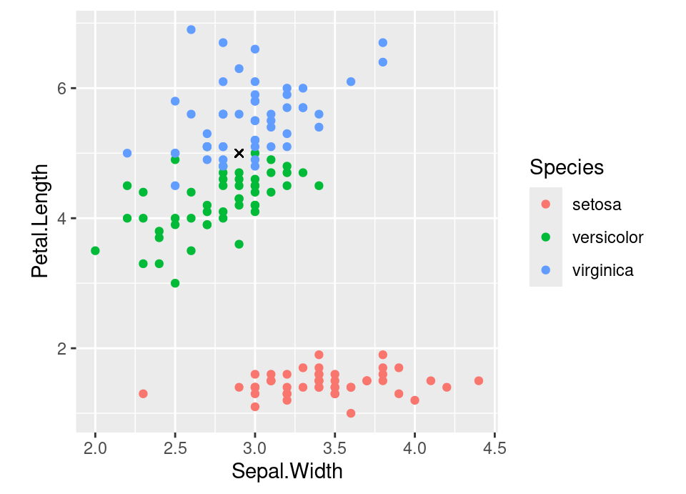
The observed data are the coloured points, with the features being the iris’ sepal width and petal length and the response represented by colour, indicating the iris species. The requirement is to predict the species of the observation with features denoted by the black cross above. Intuitively, \(k\)-nearest neighbour does what probably any reasonable person might, which is to look at what species the nearby observations are. In this case, the very closest is a versicolor, but the next nearest is virginica, whilst the next closest after that is again virginica. Therefore, the 1-nearest, 2-nearest and 3-nearest would all reach different conclusions (versicolor, a tie, or virginica). We will now formalise this.
First, given dataset \(\mathcal{D}_n = \left( (\vec{x}_1, y_1), \dots, (\vec{x}_n, y_n) \right)\), we define the reordered data with respect to the new prediction value \(\vec{x}\) by \(\left( (\vec{x}_{(1,\vec{x})}, y_{(1,\vec{x})}), \dots, (\vec{x}_{(n,\vec{x})}, y_{(n,\vec{x})}) \right)\) where \[ d(\vec{x}_{(i,\vec{x})}, \vec{x}) \le d(\vec{x}_{(j,\vec{x})}, \vec{x}) \quad \forall\, i < j\] Ties may be broken randomly; or both ties included, possibly with some re-weighting; or it may be broken by looking to the \(k+1\)-st neighbour.
Then, the knn prediction for a target loss \(\mathcal{L}(\cdot, \cdot)\) is given by considering the first \(k\) elements of the reordered dataset using the direct approximation of the Bayes optimal choice: \[\begin{align*} g^\star(\vec{x}) &= \arg\min_{z \in \mathcal{Y}} \int_\mathcal{Y} \mathcal{L}(y, z) \,d\pi_{Y \given X = \vec{x}} \\ &\approx \arg\min_{z \in \mathcal{Y}} \frac{1}{k} \sum_{i=1}^k \mathcal{L}\left(y_{(i,\vec{x})}, z\right) \end{align*}\] We know from §3.5 that this empirical estimator will carry over to have a simple form for certain loss functions. For example, for regression: \[ g^\star(\vec{x}) \approx \begin{cases} \frac{1}{k} \sum_{i=1}^k y_{(i,\vec{x})} & \text{for squared loss} \\ \text{median} \{ y_{(i,\vec{x})} : i\in\{1,\dots,k\}\} & \text{for absolute loss (odd } k \text{)} \end{cases} \] or for binary classification with 0-1 loss: \[ g^\star(\vec{x}) \approx \begin{cases} 1 & \text{if } \sum_{i=1}^k y_{(i,\vec{x})} > \frac{k}{2} \\ 0 & \text{otherwise} \end{cases} \] and so on. In particular, an empirical estimator of the probability is often taken to be, \[\mathbb{P}(Y = j \given X = \vec{x}) = \frac{1}{k} \sum_{i=1}^k \bbone\{ y_{(i,\vec{x})} = j \}\] although this has the drawback of discretising the probability in a way that depends on \(k\).
Of course, we need to choose the value \(k\), which serves as our first example of a machine learning hyperparameter: that is, a parameter which is not part of the model (ie not fitted directly on the training data) but which defines the behaviour of the model and model fit. There are generic approaches to sensible choice or amalgamation of hyperparameters which we return to in the next Chapter — for example cross-validation to choose \(k\) does lead to asymptotic consistency (Li, 1984)
Example 4.1 The code below provides an example using the gknn function in the e1071 (Meyer et al., 2021) package to predict penguin species in the Palmer penguins dataset (§B.1), using only 2 of the available variables to enable visualisation. In particular, see that appendix for the colour scheme legend used to show prediction regions.
Experiment with the code as indicated to see the behaviour of \(k\)-nearest neighbours for different settings.
# Things to explore:
#   - changing value of k on line 15
#   - using a different distance metric on line 16
#   - alter prediction point values on lines 19-20

# Package containing gknn function
library("e1071")

# Load data
data(penguins, package = "palmerpenguins")

# Fit k-nearest neighbour
fit.knn <- gknn(species ~ bill_length_mm + bill_depth_mm,
                penguins,
                k = 1,
                method = "Euclidean")

# Example prediction point (shown as a white cross on plot)
new.pt <- data.frame(bill_length_mm = 59,
                     bill_depth_mm = 17)
predict(fit.knn, new.pt, type="votes")

# Plot packages
library("ggplot2")
library("ggnewscale")

# Construct a hexagons grid to plot prediction regions
hex.grid <- hexbin::hgridcent(80,
                              range(penguins$bill_length_mm, na.rm = TRUE),
                              range(penguins$bill_depth_mm, na.rm = TRUE),
                              1)
hex.grid <- data.frame(bill_length_mm = hex.grid$x,
                       bill_depth_mm  = hex.grid$y)

# Get KNN vote predictions at the hex grid centres
hex.grid <- cbind(hex.grid,
                  predict(fit.knn, hex.grid, type = "votes"))

# Construct a column of colourings based on Maxwell's Triangle
hex.grid$col <- apply(hex.grid[,3:5], 1, function(x) {
  x <- x/max(x)*0.9
  rgb(x[1],x[2],x[3])
})
all.cols <- unique(hex.grid$col)
names(all.cols) <- unique(hex.grid$col)

# Generate plot showing training data, decision regions, and new.pt
ggplot() +
  geom_hex(aes(x = bill_length_mm,
               y = bill_depth_mm,
               fill = col,
               group = 1),
           data = hex.grid,
           alpha = 0.7,
           stat = "identity") +
  scale_fill_manual(values = all.cols,
                    guide = "none") +
  new_scale("fill") +
  geom_point(aes(x = bill_length_mm,
                 y = bill_depth_mm,
                 fill = species),
             data = penguins,
             pch = 21) +
  scale_fill_manual("Species",
                    values = c(Adelie = "red",
                               Chinstrap = "green",
                               Gentoo = "blue")) +
  geom_point(aes(x = bill_length_mm,
                 y = bill_depth_mm),
             col = "white",
             pch = 4,
             data = new.pt)
4.1.1 Bayesian \(k\)-nearest neighbour
More appealing to our statistical predilections may be a Bayesian formulation of the knn procedure. One approach to achieve this (Holmes and Adams, 2002) takes a model based on \(k\) and an additional parameter \(\beta\) which modulates the strength of effect between neighbouring observations, formulated as: \[ p(k, \beta \given \mathcal{D} = (\mat{X}, \vec{y})) \propto \mathbb{P}(Y = \vec{y} \given \mat{X}, k, \beta) p(k, \beta) \] where \[ \mathbb{P}(Y = \vec{y} \given \mat{X}, k, \beta) = \prod_{i=1}^n \frac{\exp\left( \frac{\beta}{k} \sum_{j=1}^k \bbone\{ y_i = y_{(j,\vec{x}_i)} \} \right)}{\sum_{\ell=1}^g \exp\left( \frac{\beta}{k} \sum_{j=1}^k \bbone\{ \ell = y_{(j,\vec{x}_i)} \} \right)} \] and priors are independent, \(p(k, \beta) = p(k) p(\beta)\), with default choice of uniform \(k\) on \(\{1, \dots, n\}\) and improper uniform on \(\beta \in \mathbb{R}^+\) (or a highly dispersed proper distribution). For large \(n\) the uniform on \(k\) may be truncated. Posterior predictive estimation for a newly observed \(\vec{x}_{n+1}\) is then given by: \[ \mathbb{P}(Y = y_{n+1} \given \vec{x}_{n+1}, \mat{X}, \vec{y}) = \sum_{k=1}^n \int \mathbb{P}(Y = y_{n+1} \given \vec{x}_{n+1}, \mat{X}, \vec{y}, k, \beta) p(k, \beta \given \mat{X}, \vec{y}) \, d\beta \] where \[ \mathbb{P}(Y = y_{n+1} \given \vec{x}_{n+1}, \mat{X}, \vec{y}, k, \beta) = \frac{\exp\left( \frac{\beta}{k} \sum_{j=1}^k \bbone\{ y_{n+1} = y_{(j,\vec{x}_{n+1})} \} \right)}{\sum_{\ell=1}^g \exp\left( \frac{\beta}{k} \sum_{j=1}^k \bbone\{ \ell = y_{(j,\vec{x}_{n+1})} \} \right)} \] This Bayesian approach avoids the need to specify \(k\) and, despite the flat priors, exhibits good behaviour in terms of not overfitting (see paper for details).
However, there is a significant computational price to pay (as ever!) for being Bayesian, with the posterior predictive integral evaluated either via MCMC or using numerical quadrature methods.
4.1.2 Theoretical behaviour
On the theoretically appealing side, knn is asymptotically consistent as long as the choice for \(k\) is st \(k/n \to 0\) as \(n\) increases (first shown in C. J. Stone, 1977, Corollary 3, since then conditions relaxed). However, it is theoretically less appealing that the rate of convergence of the expected error to the Bayes error in the regression setting is bounded above by an \(O\left(n^{-2\alpha/(d+2\alpha)}\right)\) term (\(f\) bounded, \(\alpha\)-Hölder continuous plus finite moment conditions on \(X\); see Kohler et al. (2006)) — notice the denominator in the exponent has power 1, meaning convergence is substantially slower as dimenion grows. This is classic “curse of dimensionality” behaviour: in other words, in the Lipschitz continuous case (ie \(\alpha=1\)) moving from a 2-dimensional to a 6-dimensional model could require squaring the available number of training observations to maintain the same accuracy, all other things being notionally equal.
Conditions such as \(\alpha\)-Hölder continuity8 are quite natural here, because it effectively bounds how quickly the function can change, which is essential for a ‘local’ method to learn anything useful from nearby observations.
Other theoretical results include the nice property that for \(k=1\) in a classification setting, no \(k>1\) has lower error against all possible distributions (Cover and Hart, 1967). However, in practical reality if we have sufficient data we typically want to choose \(k\) large enough to guard against making a non-Bayes optimal classification, but small enough that we are actually reflecting the conditional distribution \(\pi_{Y \given X = \vec{x}}\). This amounts to a bias-variance trade off: \(k=1\) has low bias but high variance, \(k \gg 1\) has higher bias but lower variance (see general discussion in the previous Chapter). There is an extensive review of finite sample theoretical results for both regression and classification settings in Chen and Shah (2018), both for \(k\) and \(n\) requirements to achieve a prescribed error, or the error achievable for a given \(k\) and \(n\).
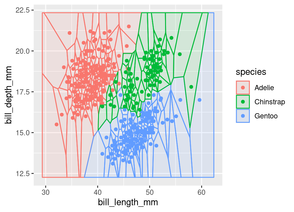
Finally, the \(k=1\) classification case is also especially interesting as it precisely corresponds to a Voronoi diagram (Aurenhammer, 1991) on the feature space, a well studied structure in computational geometry. The Voronoi diagram of a set of \(n\) points in \(\mathbb{R}^d\) consists of a partition of this space into a total of \(n\) convex \(d\)-polytopes containing only one of the points and representing the regions which are closest to the contained point. That is, the regions \(V_i \subset \mathbb{R}^d\) where \(V_i = \{ \vec{x} \in \mathbb{R}^d : d(\vec{x}_i, \vec{x}) \le d(\vec{x}_j, \vec{x}) \ \forall\, j) \}\).
The Voronoi diagram for 2 dimensions in the Palmer penguins dataset (§B.1), coloured by species follows:
4.1.3 Computational concerns
If we were to implement knn in an entirely naïve manner, we would expect to encounter two serious issues: a computational cost \(\propto nkd\) and a memory cost \(\propto nd\).
Memory: Whilst huge datasets may be efficiently summarised by regression modelling approaches which require retention of only a handful of parameters, knn lacks a fitted model: in some sense the full training data is the model. In the case of knn regression, this is difficult to tackle. However, for knn classification there have been various approaches suggested which enable reducing the memory burden, usually by either retaining points near decision boundaries and removing interior ones that appear redundant (‘condensing’, started in Hart (1968)), or conversely removing noisy points near the decision boundary to retain representative central observations (‘editing’, started in Wilson (1972)), or some combination of approaches.
Consider for example condensing. The following plot zooms into a region near the centre of the Palmer penguins dataset (§B.1) Voronoi diagram above. All points which are ‘interior’ in the sense that all their neighbouring Voronoi cells have the same colour, are indicated with a bold cross.

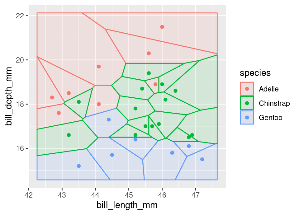
The second diagram shows that the 1-nearest neighbour rule is unaffected by removing the interior points, but memory use will be reduced because all redundancy has been eliminated by this condensing procedure. Of course for \(k>1\) the decision boundary will have been altered.
An overview of the many approaches seeking to reduce memory use in knn is in García et al. (2012).
Compute: Closely related to the memory issue is the fact that retention of so much information in order to perform a prediction leads to immense compute cost, proportional to \(nkd\), if the whole dataset is scanned. However, methods from computer science can help mitigate some of these costs. For example, perhaps most commonly used are \(k\)-d tree algorithms (Bentley, 1975) such as provided by Friedman et al. (1977), which requires one-off pre-computation \(\propto kn\log n\) to then enable on average \(\propto \log n\) cost to identify nearest neighbours for predictions. Unfortunately, this has a memory impact with space requirements which are exponential in \(d\), which has led to related more recent approaches which enable also approximate nearest neighbour computation using cover trees (Beygelzimer et al., 2006). There are other approaches seeking only approximate nearest neighbours often by deploying random projections, see Andoni et al. (2018) for an extensive recent review.
4.1.4 Curse of dimensionality
The theoretical convergence rate above, \(O\left(n^{-2\alpha/(d+2\alpha)}\right)\), is an example of the so-called ‘curse of dimensionality’. Here we try to provide a little intuition why this unattractive rate arises.
A core assumption of knn is that there the training data will contain observations that are ‘nearby’ to any future observation we wish to predict. However, as the dimensionality of a probability distribution increases the size of neighbourhoods grows dramatically.
The classic example of this is to consider the unit hypercube as our feature space \(\mathcal{X} = [0,1]^d\), with \(\pi_{X}\) being uniform on the hypercube. Taking this setting, let us examine the \(k=5\) nearest neighbours: then a measure of how truly ‘local’ these neighbours are would be given by the smallest bounding hypercube. Below is an interactive plot of 100 samples, with a red point at \((0.5,0.5,0.5)\), the 5 nearest neighbours in green and a the smallest bounding hypercube shown in transparent green.
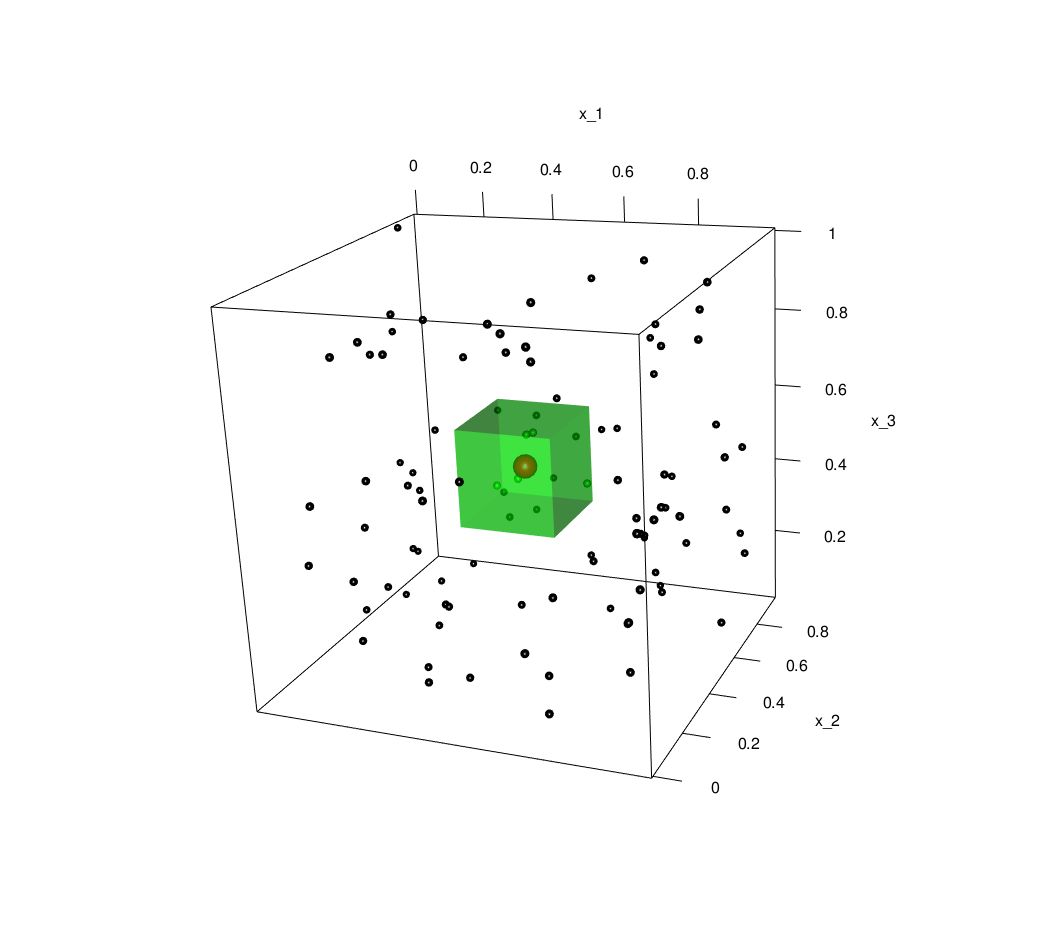
In general, let \(\ell\) be the length of the side of the bounding hypercube in \(d\) dimensional space. Then because the distribution is uniform, we have that the volume of the box should (on average) be \(\ell^d \approx \frac{k}{n} \implies \ell \approx \left( \frac{k}{n} \right)^\frac{1}{d}\). Consequently, as dimension increases for fixed samples sizes, the size of the smallest bounding box rapidly approaches the size of the whole space.
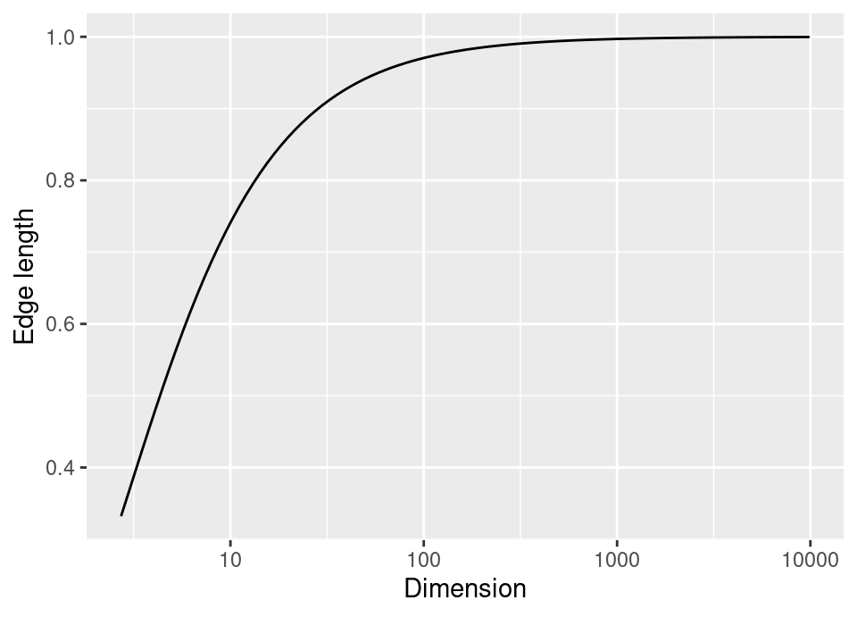
Indeed, as this plot shows, by 100 dimensions the minimal bounding hypercube around the 5 nearest neighbours with 100 training observations has edge \(\ell=0.97\), so that the box covers nearly all of \(\mathcal{X}\). In high dimensions, effectively all points are far apart and knn is not truly making predictions based on ‘local’ information.
§2.5 of Hastie et al. (2009) has further detailed discussion of this phenomenon.
4.1.5 Application considerations
Distance: The most common choices are either \(\ell_1\)-norm (Manhattan), \(\ell_2\)-norm (Euclidean) or Mahalanobis distance when in the simple setting of all numeric predictors for standard tabular data.
However, in practical applications it is common to have mixed datasets including dichotomous, qualitative and quantitative variables. A common choice in this instance is Gower’s distance (Gower, 1971). Here, to compute \(d(\vec{x}_i, \vec{x}_j)\), take each variable, \(\ell \in \{1, \dots, d\}\) and depending on whether it is numeric or categorical:
- Numeric: \(\delta_\ell = \frac{|x_{i\ell}-x_{j\ell}|}{R_\ell}\) where \(R_\ell = \max_i \{x_{i\ell}\} - \min_i \{x_{i\ell}\}\)
- Categorical: \(\delta_\ell = \begin{cases} 1 & \text{if } x_{i\ell}=x_{j\ell} \\ 0 & \text{otherwise} \end{cases}\)
The total distance is then computed as the simple average, \(d(\vec{x}_i, \vec{x}_j) = \frac{1}{d} \sum_{\ell=1}^d \delta_\ell\)
There are other settings, such as data that is not standard tabular data (eg images) where often completely custom distances are employed. For example, in image data there is no reason to believe only the exact pixel activations are relevant, but that translation, scaling and limited rotation of training data should lead have the same response. §13.3.3 in Hastie et al. (2009) is a very nice example of this for image data.
Scaling: A problem with \(k\)-nearest neighbours is that the prediction is not invariant to the scale of individual variables. Therefore, it is fairly standard practice to centre (subtract mean) and scale (divide by standard deviation) the training data. Note that one must then also centre and scale the data to be predicted. Crucially, you must use training data mean and standard deviation for scaling the features of the new point to predict!
4.1.6 Further reading
Barber (2012), §14.3, provides a generative probabilistic model interpretation of knn; Bach (2021), Ch.6, provides accessible coverage of key theory; for a more exhaustive coverage, Chen and Shah (2018) provides a monograph length review many aspects of nearest-neighbour methods.
A large scale and relatively recent example application of \(k\)-nearest neighbours was the first ever attempt to geolocate a photograph to a GPS position on the surface of the Earth by Hays and Efros (2008), which used a database of over 6 million images and a 120-nearest neighbour algorithm.
4.2 Smoothing kernel approaches
The first local method we saw, \(k\)-nearest neighbours, produced an empirical estimator by defining that another observation is ‘local’ by a threshold on the number of observations, irrespective of how far the most distant of those \(k\) neighbours is (ie fixed number of neighbours, dynamically adjusting distance). Therefore in densely populated areas of the training data feature space, points considered ‘local’ are much closer than in sparsely populated regions of feature space.
What may be thought of as a dual of this idea is to instead define the local region by a fixed distance and consider only observations within that distance to be ‘local’ (ie dynamic number of neighbours, fixed distance). This would be trivially achievable using the indicator function, for example in the regression setting with some distance \(d : \mathcal{X} \times \mathcal{X} \to [0,\infty)\), \[ \hat{f}(\vec{x}) = \frac{\sum_{i=1}^n y_i \bbone\{ d(\vec{x}_i, \vec{x}) < h \}}{\sum_{i=1}^n \bbone\{ d(\vec{x}_i, \vec{x}) < h \}} \]
Now instead of specifying \(k\), we specify \(h \in \mathbb{R}^+\), which is usually referred to as the bandwidth. In practice, we could consider a more general form of this idea, which provides a smoother estimate than the indicator function above. This idea of defining locality by distance (in a possibly smooth way) then leads to natural approaches to all three problem types described in the problem setting. Note that detailing these techniques could occupy an entire course by itself: the treatment here will be brief. The monograph by Silverman (1998) provides a gentle introduction to key background.
4.2.1 Kernel density estimation
We address the third problem type from the problem setting first — that is the problem of general density estimation — the other approaches then following naturally from it. That is, we wish to construct a density estimator of some distribution \(\pi_X\) (by natural extension, \(\pi_{XY}\)).
The simplest density estimator everyone will be familiar with is a histogram estimator, which takes fixed bins and constructs an empirical estimate of the density by the proportion of observations falling in each bin. The most naïve extension of this concept does not have fixed bin placement, but builds up the estimator by accumulating bins centred on the observations themselves. We can see this is justified by relation of the probability density function, \(f_X(x)\), to the cumulative distribution function, \(F_X(x)\), in the simple 1-dimensional case as follows,
\[\begin{align*} f_X(x) &= \frac{\partial F_X}{\partial x}(x) \\ &= \lim_{h \to 0} \frac{F_X(x+h) - F_X(x)}{h} \\ &\equiv \lim_{h \to 0} \frac{F_X(x) - F_X(x-h)}{h} \\ \implies \frac{f_X(x)+f_X(x)}{2} &= \lim_{h \to 0} \frac{F_X(x+h) - \cancel{F_X(x)} + \cancel{F_X(x)} - F_X(x-h)}{2h} \\ f_X(x) &= \lim_{h \to 0} \frac{\mathbb{P}(x-h < X < x+h)}{2h} \\ &\approx \frac{1}{2h} \left(\frac{1}{n} \sum_{i=1}^n \bbone\{ x-h < x_i < x+h \}\right) \text{ for small } h>0 \\ &= \frac{1}{n} \sum_{i=1}^n \underbrace{\frac{1}{2h} \bbone\left\{ \left| \frac{x-x_i}{h} \right| < 1 \right\}}_{\star \ \text{valid uniform pdf}} \end{align*}\]where we have data \((x_1, \dots, x_n)\) which are iid realisations of \(X\) used to provide an empirical estimate of the required probability. Note in particular that the term \(\star\) within the sum on the final line is a valid uniform probability density function.
The following plot shows this estimator for the first 50 Palmer penguins flipper lengths. The coloured bottom row shows \(\frac{1}{n}\times\) each term in the sum, with the solid black line showing the full density estimator, with \(h=1\).
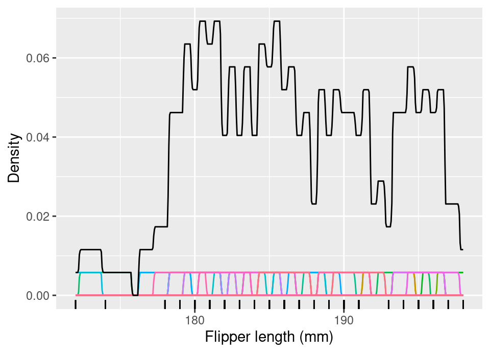
This density estimator is rather rough, even though it improves on a histogram estimate by avoiding fixed bin positioning. This can be made ‘smoother’ by considering the class of so-called kernel functions as a replacement for the uniform density within \(\star\), which will lead to a kernel density estimator (KDE). Intuitively, this amounts to placing a ‘hump’ of probability on each observation, by centring the mean of some pdf on each observation and scaling the density value by \(\frac{1}{n}\), thereby ensuring the sum of all ‘humps’ results in a valid pdf. For example, the above corresponds to a uniform pdf on \([-1,1]\), rescaled to \([-h,h]\), centred at each \(x_i\) and with density value scaled by \(\frac{1}{n}\).
It appears the ideas leading to kernel density estimation were initially formed in Rosenblatt (1956), Whittle (1958) and Parzen (1962).
Definition 4.1 (Kernel function) A kernel function9 is any function \(K\) such that,
- \(K : \mathcal{X} \to [0,\infty)\)
- \(K(\cdot)\) is a valid probability density (integrating to 1), \[ \int_\mathcal{X} K(d\pi_X) = 1\]
- \(K(\cdot)\) is symmetric, \(K(\vec{x}) = K(-\vec{x}) \ \forall\, \vec{x} \in \mathcal{X}\).
Some authors only require (i) or (i) and (ii), whilst others add explicit moment conditions on \(K(\cdot)\) (ie second moment =1, all moments finite).
There is of course the issue of scaling the kernel to match \(h\), the so-called bandwidth. Therefore, we have in general the following form for a KDE.
Definition 4.2 (Kernel density estimator) The kernel density estimator of the density \(f_X(\cdot)\) based on \(n\) iid observations \((\vec{x}_1, \dots, \vec{x}_n)\) drawn from \(\pi_X\) is given by: \[ \hat{f}_X(\vec{z}) = \frac{1}{n} \sum_{i=1}^n \frac{1}{h^d} K\left(\frac{\vec{z}- \vec{x}_i}{h}\right) \] Note that this results in \(\hat{f}_X(\vec{z})\) being a valid probability density function.
In many cases, it is often simpler to construct the estimator as a product of univariate densities, so you may see this written instead as, \[ \hat{f}_X(\vec{z}) = \frac{1}{n} \sum_{i=1}^n \prod_{\ell=1}^d \frac{1}{h_\ell} K\left( \frac{z_\ell-x_{i\ell}}{h_\ell} \right) \] with now \(K : \mathbb{R} \to [0,\infty)\) and with possibly different bandwidths in each dimension, \(h_\ell\).
Example 4.2 (Common kernel functions) Using the univariate construction above, common kernel functions include (see after for visualisation):
Епанечников (1969) (translation Epanechnikov (1969)) \[ K(x) = \frac{3}{4}(1-x^2) \bbone\{ |x| \le 1 \} \] though the original presentation was scaled by a factor \(\sqrt{5}\) to have unit second moment (and is otherwise identical), \[ K(x) = \left(\frac{3}{4 \sqrt{5}} - \frac{3 x^2}{20 \sqrt{5}}\right) \bbone\{ |x| \le \sqrt{5} \} \]
Gaussian \[ K(x) = \frac{1}{\sqrt{2 \pi}} \exp\left( \frac{x^2}{2} \right) \]
Triangular \[ K(x) = (1 - |x|) \bbone\{ |x| \le 1 \} \]
Practically speaking, any of these choices (and more) do not have much impact on the results.
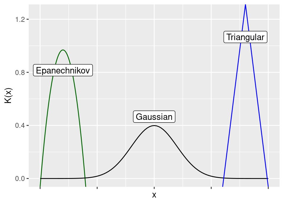
There is a small advantage which motivates the Epanechnikov kernel, because it is the theoretically optimal choice of univariate product kernel, in terms of asymptotically minimising expected squared loss between the estimated and true densities (Epanechnikov, 1969; Епанечников, 1969). The advantage is so small that in applications other considerations dominate.
The following plot shows the same first 50 Palmer penguins flipper lengths used for density estimation, with columns showing different kernel functions and rows different choices for \(h\).
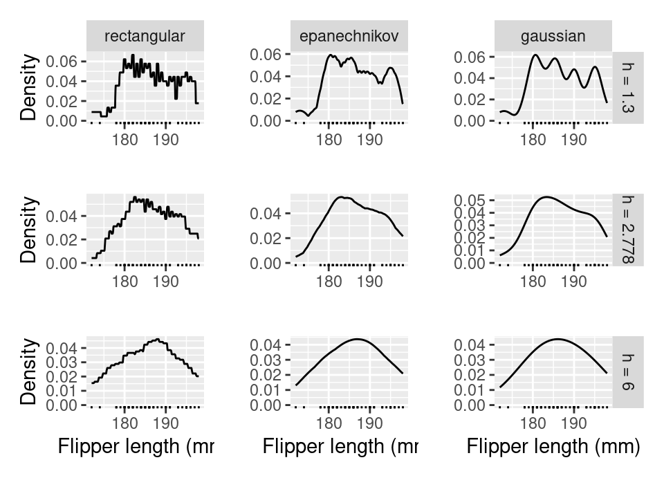
The middle row has estimated optimal value \(h=2.778\), computed using the method of Sheather and Jones (1991) (see §4.2.1.2 below for brief discussion).
You can explore different kernels and bandwidths to observe the behaviour using the following code:
library(ggplot2)

# Load penguins data and just use first 50 observations
data(penguins, package = "palmerpenguins")
x <- na.omit(penguins$flipper_length_mm)

# Look at a bog standard histogram first
hist(x)

# Compute the kernel density estimate
dens <- density(x, bw = 2.7, kernel = "epanechnikov")

# Plot with base R
plot(dens)

# Alternatively, we can compute the density estimate and plot simultaneously with ggplot
ggplot(data.frame(flipper_length_mm = x)) +
  geom_density(aes(x = flipper_length_mm),
               bw = 2.7,
               kernel = "epanechnikov") +
  geom_rug(aes(x = flipper_length_mm)) +
  ylab("Density") +
  xlab("Flipper length (mm)")
4.2.1.1 Theoretical behaviour
Kernel density estimation is about density estimation in the most general sense, and not only in the framework of the problem setting from the last Chapter. Therefore, the theoretical analysis focuses on subtly different (but very closely related) quantities to those discussed before (see Grund et al. (1994) for perspectives on loss/risk in the kernel density setting).
The two main quantities analysed are, \[\begin{align*} &\mathbb{E}_{\pi_X^n}\left[\left( f_X(\vec{x}) - \hat{f}_X(\vec{x}) \right)^2\right] & \quad \text{ mean square error (MSE)} \\ \int_\mathcal{X} &\mathbb{E}_{\pi_X^n}\left[\left( f_X(\vec{x}) - \hat{f}_X(\vec{x}) \right)^2\right] \,d\vec{x} & \quad \text{ mean integrated square error (MISE)} \end{align*}\]
Note that the MSE is computed for a fixed \(\vec{x}\). Note also that the MISE integrates over \(\vec{x}\), but not with respect to \(\pi_X\) as a base measure (ie subtley different to expected error, so that for example tail discrepancies matter as much as those in the regions of high probability: what you would want if the whole density is of interest and not prediction on the basis of new draws from it).
These possess a bias/variance decomposition (analogous to the regression setting in Example 3.8) and, for example, lead to an asymptotic analysis in 1D on the MSE (see Rosenblatt (1971) (eq 15+16) for derivation and full conditions) which shows, \[\begin{align*} \text{Bias}[\hat{f}_X(x)] &\approx \frac{h^2}{2} f''_X(x) \int z^2 K(z) \,dz + o(h)^2 = O\left(h^2\right) \\ \text{Var}[\hat{f}_X(x)] &\approx \frac{f_X(x)}{nh} \int K^2(z) \,dz = O\left((nh)^{-1}\right) \end{align*}\]
This means that the bandwidth \(h\) controls the classical bias-variance trade-off, where large \(h\) leads to high bias and low \(h\) leads to high variance, with the optimal bandwidth shrinking at a rate order \(n^{-1/5}\) in sample size. This results in the MSE converging to zero at a rate \(n^{-4/5}\).
Put together, one arrives at asymptotic mean integrated square error, \[\text{AMISE} = \frac{1}{nh} \int K^2(z) \,dz + h^4 \left( \int f''_X(z)^2 \,dz \right) \left( \int z^2 K(z) \,dz \right)^2\]
Finally, KDE is consistent (Parzen, 1962) if \(nh \to \infty\) as \(n \to \infty\) and \(h \to 0\) (ie \(h = h(n)\) varies with sample size). Note that here, consistency is in MSE as defined above, so is pointwise unlike the standard ML definition from the previous chapter.
4.2.1.2 Bandwidth selection
One then has two choices: seek a bandwidth which is optimal for estimation at a particular \(x\) (ie choose \(h\) to minimise MSE), or make a global choice (ie choose \(h\) to minimise MISE). For example, in the global setting one can conclude the theoretically optimal bandwidth is,
\[ h = \left( \frac{\int K^2(z) \,dz}{n \left( \int f''_X(z)^2 \,dz \right) \left( \int z^2 K(z) \,dz \right)^2} \right)^\frac{1}{5}\]
We see that if \(f\) changes rapidly then \(f''\) will be large, leading to a smaller \(h\) (due to the integrated \(f''\) in the denominator) in order to capture rapidly changing structure. Likewise the other integral in the denominator provides the squared second moment of the kernel being used (ie squared variance if it has zero mean), so that high variance kernels are compensated with smaller bandwidth.
Unfortunately, the optimal bandwidth is impossible to compute because we do not know \(f''_X(\cdot)\) and therefore do not know the measure of overall roughness (it is worse in the non-global setting where we need to know \(f_X\) and \(f''_X\) for all \(x\)). However, we can conclude that rougher probability density functions and larger sample sizes will need smaller choices of bandwidth.
Despite this, the above theoretical solution has led to a number of methods which attempt to provide automatic methods for choosing \(h\), including:
- Rules of thumb which just estimate \(\int f''_X(z)^2 \,dz\) by substituting the result of this integral by the value obtained if \(f_X\) was a Normal density. This is the default method used by the
density()function in R. - Cross validation (see next chapter) based estimates, either unbiased or biased. Call
density(..., method = "ucv")ordensity(..., method = "bcv")in R to use these estimates. - Plug-in approaches, which make a pilot estimate of the derivative and then attempts to solve the above equation by seeking the fixed-point. Call
density(..., method = "SJ")in R to use this estimate.
For full details and original references see the excellent survey in Jones et al. (1996), where the plug-in approach (method = "SJ") is recommended.
It is beyond our scope here, but note there have also been attempts to look at locally adaptive bandwidth choices (rather than a single global choice above). See in particular the sequence of papers Breiman et al. (1977), Abramson (1982), and Terrell and Scott (1992).
Finally, note that the standard scalar bandwidth can be replaced with a symmetric positive definite \(d \times d\) bandwidth matrix \(\mat{H}\), with the estimator becoming: \[ \hat{f}_X(\vec{z}) = \frac{1}{n} \sum_{i=1}^n |\mat{H}|^{-\frac{1}{2}} K\left( \mat{H}^{-\frac{1}{2}} (\vec{z}- \vec{x}_i) \right) \] though in reality the simplifying assumption that \(\mat{H}\) is diagonal is made, reducing to the product estimate above.
4.2.2 Nadaraya-Watson estimator
With the above slight detour, we are able to return to the primary focus and use these methods to develop local regression and classification estimators based on kernels (rather than nearest neighbours) to define locality.
The Nadaraya-Watson estimator (Nadaraya, 1964; Watson, 1964) is based on an elegantly simple kernel density approximation to the necessary conditional distribution. As discussed at the start of this chapter, local methods attempt to directly estimate the Bayes optimal predictor empirically, so in a regression context we want to directly estimate \(\mathbb{E}\left[ Y \given X = \vec{x} \right]\).
\[\begin{align*} \mathbb{E}\left[ Y \given X = \vec{x} \right] &= \int_\mathcal{Y} y f_{Y \given X}(y \given \vec{x}) \,dy \\ &= \int_\mathcal{Y} y \frac{f_{XY}(\vec{x}, y)}{f_{X}(\vec{x})} \,dy \\ &\approx \int_\mathcal{Y} y \frac{\cancel{\frac{1}{n}} \sum_{i=1}^n \frac{1}{h^{d+1}} K\left(\frac{\vec{x}- \vec{x}_i}{h}\right) K\left(\frac{y- \vec{y}_i}{h}\right)}{\cancel{\frac{1}{n}} \sum_{i=1}^n \frac{1}{h^d} K\left(\frac{\vec{x}- \vec{x}_i}{h}\right)} \,dy \\ &= \frac{\sum_{i=1}^n \cancel{\frac{1}{h^d}} K\left(\frac{\vec{x}- \vec{x}_i}{h}\right) \int_\mathcal{Y} \frac{y}{h} K\left(\frac{y- \vec{y}_i}{h}\right) \,dy}{\sum_{i=1}^n \cancel{\frac{1}{h^d}} K\left(\frac{\vec{x}- \vec{x}_i}{h}\right)} \\ &= \frac{\sum_{i=1}^n y_i K\left(\frac{\vec{x}- \vec{x}_i}{h}\right)}{\sum_{i=1}^n K\left(\frac{\vec{x}- \vec{x}_i}{h}\right)} \end{align*}\]where the \(\approx\) follows by creating kernel density estimates of numerator and denominator (\(f_{XY}(\vec{x}, y)\) using the product of kernels estimate discussed earlier), and with the integral on the next line simply being the expectation with respect to the pdf \(h^{-1} K\left(\frac{y- \vec{y}_i}{h}\right)\), which is symmetric and centred at \(y_i\).
Definition 4.3 (Nadaraya-Watson estimator) The kernel based Nadaraya-Watson estimator of a regression function based on training data \(\mathcal{D}_n = \left( (\vec{x}_1, y_1), \dots, (\vec{x}_n, y_n) \right)\) is: \[ \hat{f}(\vec{x}) = \frac{\sum_{i=1}^n y_i K\left(\frac{\vec{x}- \vec{x}_i}{h}\right)}{\sum_{i=1}^n K\left(\frac{\vec{x}- \vec{x}_i}{h}\right)} \]
Selection of the bandwidth remains an issue here and is typically harder to select than in the density estimation setting. We will visit cross-validation in the next chapter which is commonly used and, for leave-one-out, is consistent (Wong, 1983). There also exist plug-in estimators (Wand and Jones, 1995).
A simple extension of the Nadaraya-Watson estimator idea often gives better results: the local polynomial estimator (see eg Hastie et al. (2009)).
The standard Nadaraya-Watson estimator can be fitted using ksmooth() in base R, whilst local polynomial estimators are available in KernSmooth::locpoly() (Wand, 2021). See the following live code:
TODO: live code here
4.2.2.1 Further reading
The monograph Wand and Jones (1995) also has excellent coverage of local polynomial estimators.
4.2.3 Kernel density classification & naïve Bayes
It is also possible to apply kernel density estimation in the classification case. In particular, in it a simple application of Bayes’ Theorem to transform the classification problem into the generative modelling form (raised in the last Chapter):
\[ \mathbb{P}(Y = i \given X = \vec{x}) = \frac{f_{X \given Y}(\vec{x} \given Y = i) \mathbb{P}(Y = i)}{\sum_{j=1}^g f_{X \given Y}(\vec{x} \given Y = j) \mathbb{P}(Y = j)} \]
where now \(f_{X \given Y}(\vec{x} \given Y = i)\) is simply a target density we may choose to estimate via kernel density estimation. It is then a simple plug-in estimate where we replace \(f_{X \given Y}(\vec{x} \given Y = i)\) with the kernel density estimate, and replace \(\mathbb{P}(Y = i)\) with the empirical estimator of the prevalence of label \(i\) (Aitchison and Aitken, 1976).
However, we know this can be problematic in high dimensional problems where we have many features. The problem is therefore simplified by making the so-called naïve Bayes assumption (the earliest example I can find of this assumption is actually in the medical literature Warner et al. (1961)).
Definition 4.4 (Naïve Bayes classifier) The naïve Bayes classifier is formed by constructing a generative model for the classification problem, but with the assumption of conditional independence of all dimensions in \(\mathcal{X}\). That is, we assume \[ \mathbb{P}(Y = i \given X = \vec{x}) = \frac{\mathbb{P}(Y = i) \prod_{k=1}^d f_{X_k \given Y}(x_k \given Y = i)}{\sum_{j=1}^g \mathbb{P}(Y = i) \prod_{k=1}^d f_{X_k \given Y}(x_k \given Y = i)} \] and construct estimates of the univariate marginal densities \(f_{X_k \given Y}(x_k \given Y = i) \ \forall\,k\).
Note that there is nothing in the definition of the naïve Bayes classifier which dictates how the univariate marginal densities are estimated. In the context of this section, it is natural to use kernel density estimation which we know can perform well in 1-dimension, but in fact many applications simply fit a Normal distribution via maximum likelihood separately for each dimension. Thus, again, this is a local method which directly constructs an empirical estimate of the Bayes optimal predictor.
The designation “naïve” is unfortunate: although the conditional independence assumption is often untrue, this approach can work well in practice (Hand and Yu, 2007; Ng and Jordan, 2001). To understand this, note that although the incorrect assumption results in the product of univariate kernels introducing bias, the very fact that these are only univariate kernel density estimates means the variance of the estimator is substantially lower than a joint high-dimensional KDE would exhibit. In many cases this trade-off can result in reduced error overall, whether estimating the marginals with KDE or a parametric method (Friedman, 1997).
You can fit in R using naivebayes::naive_bayes(..., kernel = TRUE) (Majka, 2019). The default will actually assume marginals are Gaussian, so the kernel argument needs to be provided to override this.
TODO: live code here
4.3 Further topics
This is just a taster of some local methods: it is recommended to also cover smoothing splines, an excellent resource being Chapter 5 of Hastie et al. (2009).
References
If one wishes to be pedantic, in some sense every model uses information local to \(\vec{x}\) when making predictions at that value, but what distinguishes what we refer to as local methods is that the estimation typically directly depends on the local data and not on a previously globally fitted model.↩︎
Recall briefly, a function \(f : \mathbb{R}^d \to \mathbb{R}\) is \(\alpha\)-Hölder continuous if \(\exists\) \(M, \alpha > 0\) such that \(|f(x)-f(y)| \le M \| x-y \|^\alpha\).↩︎
not to be confused with kernels used to replace inner products in kernel machines (eg SVMs).↩︎