Chapter 5 Error Estimation and Model Selection
We should no longer defer addressing arguably among the most consequent aspects of a statistical machine learning analysis: estimation of the errors the model makes and sensible selection of models. There is little benefit in deeply understanding sophisticated methods without deeply understanding sound approaches to compare them and understand future performance.
The first major reason good error estimation matters is because we saw in Chapter 3 that computing the estimated generalisation error using the same data as used to fit the model results in downward biased estimation. If we are interested in the actual error rate of the model for future predictions then clearly accurate and unbiased estimation are of interest.
A second major reason error estimation matters is in selection of so-called hyperparameters. We saw two examples of hyperparameters in local methods (the number of nearest neighbours and the bandwidth) — there is no universal agreement on the precise definition of this term, but herein we use it to describe any parameter which is not part of the model fitting process itself (ie not part of the maximum likelihood/posterior estimation or empirical risk minimisation of the model), but which must be separately ascertained somehow. This is a form of model tuning.
A third major reason is that in applications it is not uncommon use multiple different modelling approaches and then attempt to identify which one to retain as the final model. This is model selection (though sometimes we may prefer to actually use all models in an ensemble, see Chapter 7)
Note that we require the estimate of the error to be accurate in only the first case. In the second and third cases we only need a consistent estimate, in the sense that we correctly order the performance of different models. We will see this distinction matters as some methods provide only consistent estimates. Note this is the sense in which the word ‘consistent’ is used in this Chapter (it is often used in model selection to mean selection of the ‘true’ model, but our interest here is predictive performance).
There are multiple possible strategies which can be employed when estimating the errors in a fitted model. You will have seen some of these ideas in the APTS Statistical Modelling course (Kosmidis et al., 2025), but our presentation here will have a different and complementary emphasis, so do not skip this Chapter even if you studied that module. Finally, it is important to note that we will often rely on additional metrics of model performance aside from the loss, some of which we discuss in Chapter 7. Identifying the appropriate error estimates and model metrics to examine is something of an art.
5.1 In-sample estimation
As discussed in Chapter 3 at the end of the section on generalisation error, it might be tempting to try to compute some estimate of the error using the data that trained the model. In particular, we may try to approximate the total expected in-sample loss:
\[ \text{Err} := \sum_{i=1}^n \underbrace{\mathbb{E}_{Y \given X = \vec{x}_i}\left[ \mathcal{L}(Y, g_{\hat{f}}(\vec{x}_i)) \right]}_{\text{Err}_i} \]
with
\[ \text{err} := \sum_{i=1}^n \underbrace{\mathcal{L}(y_i, g_{\hat{f}}(\vec{x}_i))}_{\text{err}_i} \]
For example, in a regression setting \(\text{err}\) is the observed residual sum of squares. However, as previously discussed, this is a downward biased estimate and so we may write:
\[ \text{Err} = \text{err} + \omega \]
where \(\omega\) is called the optimism of the apparent error. A natural question is: can we estimate \(\hat{\omega} \approx \omega\) without having to collect additional data (or split up the data we do have)? If so, then it might seem we could use the approximation \(\widehat{\text{Err}} = \text{err} + \hat{\omega}\) for error estimation, hyperparameter tuning and model selection.
5.1.1 Mallows’ \(C_p\)
Mallows (1973) derived an answer to a scaled version of the above problem in the specific case of standard linear regression with homoskedastic Normal errors, \((Y \given X = \vec{x}) \sim \text{N}(\vec{x}^T \vecg{\beta}, \sigma^2)\), using squared loss:
\[C_p = \frac{\sum (y_i - \vec{x}_i^T \hat{\vecg{\beta}})^2}{\sigma^2} - n + 2d\]
Most commonly it is used as a guide to selecting which predictors to retain in a regression model (ie drop certain columns of \(\mat{X}\), refit \(\hat{\vecg{\beta}}\) and recompute \(C_p\) with the changed residual sum of squares and dimension \(d\)). The value \(\sigma^2\) must be estimated from the data, usually from the full model, and a modified \(C_p\) might be preferable in this case if using for variable selection (Gilmour, 1996).
Note that in this setting (all expectations with respect to \(\pi_{Y \given X = \vec{x}_i}\))
\[\begin{align*} \text{Err}_i &= \mathbb{E}\left[ \mathcal{L}(Y, g_{\hat{f}}(\vec{x}_i)) \right] \\ &= \mathbb{E}\left[ (Y - \vec{x}_i^T \hat{\vecg{\beta}})^2 \right] \\ &= \mathbb{E}[Y]^2 - 2 \vec{x}_i^T \hat{\vecg{\beta}} \mathbb{E}[Y] + (\vec{x}_i^T \hat{\vecg{\beta}})^2 \\ &= (\vec{x}_i^T \vecg{\beta})^2 + \sigma^2 - 2 (\vec{x}_i^T \hat{\vecg{\beta}}) (\vec{x}_i^T \vecg{\beta}) + (\vec{x}_i^T \hat{\vecg{\beta}})^2 \\ &= \left(\vec{x}_i^T \vecg{\beta} - \vec{x}_i^T \hat{\vecg{\beta}}\right)^2 + \sigma^2 \end{align*}\]Mallows (1973) proved that \(C_p\) is an unbiased estimator for \(\sigma^{-2} \sum \left(\vec{x}_i^T \vecg{\beta} - \vec{x}_i^T \hat{\vecg{\beta}}\right)^2\). Therefore, \(\sigma^2 C_p \approx \text{Err} - n \sigma^2\), implying that \(\hat{\omega} \approx 2 d \sigma^2\). This motivates an alternative form10 of Mallows’ \(C_p\), written:
\[ \tilde{C}_p = \text{err} + 2d\sigma^2 \]
Mallows’ result in fact applies to any linear estimation rule of the form \(\hat{\vec{y}} = \mat{M} \vec{y}\) (Efron, 2004), where \(\mat{M}\) does not depend on \(\vec{y}\). For example, \(\mat{M} = \mat{X} (\mat{X}^T \mat{X})^{-1} \mat{X}^T\) for standard linear regression. In this setting, the contribution to the optimism of the \(i\)th observation is \[\hat{\omega}_i = 2 \sigma^2 M_{ii}\] so that an unbiased estimate of the error above is \[\widehat{\text{Err}} = \text{err} + 2 \sigma^2 \,\text{trace}(\mat{M})\] where \(\sigma\) must also be estimated. The quantity \(\text{trace}(\mat{M})\) is now quite commonly referred to as the degrees of freedom (df) (Tibshirani, 2015).
Note that with the linear estimation formulation above, we can therefore apply this in the regression setting for both \(k\)-nearest neighbour and Nadaraya-Watson regression.
Example 5.1 (Other linear estimators) KNN: Let the matrix \(\mat{M}\) be defined by the entries:
\[ M_{ij} = \begin{cases} \frac{1}{k} & \text{if } d(\vec{x}_i, \vec{x}_j) \le d(\vec{x}_i, \vec{x}_{(k,\vec{x}_i)}) \\ 0 & \text{otherwise} \end{cases} \]
where \(\vec{x}_{(k,\vec{x}_i)}\) is as defined in the last chapter. Then, the in-sample nearest neighbour prediction of the full vector of responses \(\vec{y}\) is given by \(\hat{\vec{y}} = \mat{M} \vec{y}\) and knn may be seen as a linear estimation rule.
Nadaraya-Watson: Let the matrix \(\mat{M}\) be defined by the entries:
\[ M_{ij} = \frac{K\left(\frac{\vec{x}_i - \vec{x}_j}{h}\right)}{\sum_{\ell=1}^n K\left(\frac{\vec{x}_i - \vec{x}_\ell}{h}\right)} \]
Then, the in-sample Nadaraya-Watson prediction of the full vector of responses \(\vec{y}\) is given by \(\hat{\vec{y}} = \mat{M} \vec{y}\) and Nadaraya-Watson may be seen as a linear estimation rule.
Others: The same framework encompases many other methods which can be expressed in this form such as ridge regression, lasso, group lasso, and spline smoothing (Arlot and Bach, 2009).
5.1.2 Akaike Information Criterion (AIC)
Akaike (1972) intended to extend the concept of standard maximum likelihood by examining the maximum of the expected log-likelihood (expectation being taken with respect to the true but unknown density) for each possible model. More precisely, if we take \(\hat{\vecg{\theta}}\) to be the maximum likelihood estimate for a given model, we would examine:
\[ \mathbb{E}_{X}[\log f_X(X \given \hat{\vecg{\theta}})] = \int_\mathcal{X} \log f_X(x \given \hat{\vecg{\theta}}) d\pi_X = - \mathcal{E}\left(\hat{f}(\cdot\given\hat{\vecg{\theta}})\right)\]
and choose that fitted model for which this is maximised among all candidate models.
This corresponds to minimising the generalisation error when using a log-likelihood loss and full probabilistic model (or equal to \(\text{Err}_i\) in a fixed inputs case at some predictor). Of course, the expectation cannot be computed since the true density is unknown, although we can empirically estimate it. Maximising the above expectation is equivalent to maximising
\[ \mathbb{E}_{X}\left[ \log \frac{f_X(X \given \hat{\vecg{\theta}})}{\pi_X(X)} \right] = \int_\mathcal{X} \log \frac{f_X(x \given \hat{\vecg{\theta}})}{\pi_X(x)} d\pi_X \]
which is the Kullback-Leibler (KL) mean information for discrimination between the true model (\(\pi_X = f(\cdot \given \vecg{\theta})\)) and the fitted model (\(f_X(\cdot \given \hat{\vecg{\theta}}))\)), and for us corresponds to \(-\mathcal{E}\left(\hat{f}(\cdot\given\hat{\vecg{\theta}})\right) + \mathcal{E}\left(\pi_X\right)\), or the negative excess risk compared to the true model. By conducting an asymptotic expansion around the unknown true parameter, \(\vecg{\theta}\), and then considering only differences between models (to eliminate the dependence on the true model), Akaike (1972) derives the AIC:
\[ \text{AIC} = -2 \left(\sum_{i=1}^n \log f_X(\vec{x}_i \given \hat{\vecg{\theta}}) \right) + 2d \]
where \(d\) is the dimension of \(\vecg{\theta}\). Note that being based on the likelihood, the AIC can be used wherever there is a probabilistic model formulated11. The AIC value is therefore related to expected prediction error, and in particular it provides an estimator of the true generalisation error (Akaike, 1974):
\[\text{AIC} \approx 2 n \mathbb{E}\left[\mathcal{E}\left(\hat{f}(\cdot\given\hat{\vecg{\theta}})\right)\right]\]
In other words, the optimism of the empirical negative log-likelihood for a log-likelihood loss is approximately \(d\).
When used for model selection/hyperparameter tuning we select the model with smallest AIC. Unfortunately, AIC does not asymptotically select the ‘true’ model (and if being used for variable selection tends to choose too many predictors). However, it is asymptotically consistent in choosing a model which offers equivalent loss to the smallest available among all candidate models (Yang, 2005), which we would hope for given the above discussion. In the statistical machine learning setting where prediction is the goal, we should therefore tend not to worry that the ‘true’ model is not chosen since that is not our primary objective!
If you are more worried about scientific modelling and discovery of a ‘true’ model, then the Bayesian Information Criterion (BIC) is a better choice and does asymptotically select the ‘true’ model if the real data generating process is among the candidate models (we do not cover it here as that is not our focus for this course). Furthermore, in a statistical machine learning setting we are unlikely to believe we have an actual generative model reflecting reality in our candidate set, so in our setting BIC tends to under-perform relative to AIC for predictive performance, because it selects models that are too parsimonious. See for example Yang (2005) and references therein for theoretical proofs of these properties.
5.1.3 General covariance penalties
The two above cases bear individual attention as common in-sample estimators used most often for model selection. As demonstrated above they also provide direct estimates of training error optimism. However, Efron (1986) generalised the framework for analysing optimism in the apparent error by defining the so-called \(q\)-class of losses.
Definition 5.1 (q-class loss) A loss is said to be a \(q\)-class loss if it can be written, for some concave function \(q(\mu) : \mathcal{Y} \to \mathbb{R}\), as
\[ \mathcal{L}(y, \hat{y}) = q(\hat{y}) + \left.\frac{d q}{d \mu}\right|_{\mu = \hat{y}} (y - \hat{y}) - q(y) \]
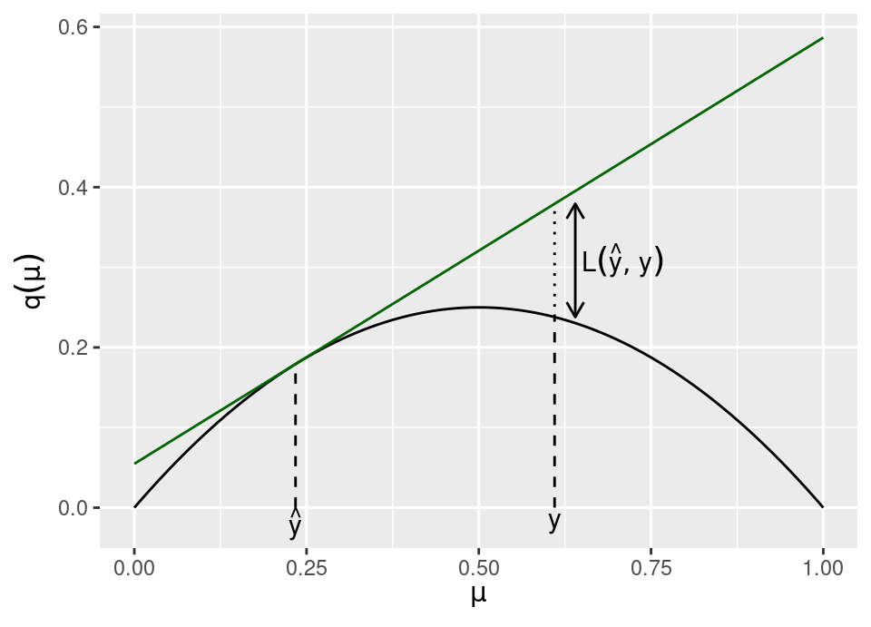
The above figure shows how to visualise losses of this class, with \(q\) being the solid black line, having tangent in dark green at \(\hat{y}\). The loss is then the difference between the \(q\) function and tangent at \(y\).
Example 5.2 (Common q-losses) Many standard losses we have encountered belong to the \(q\)-class, including:
- squared loss (shown in plot above): \[q(\mu) = \mu(1-\mu) \implies \mathcal{L}(y, \hat{y}) = (y-\hat{y})^2\]
- 0-1 loss: \[q(\mu) = \min\{\mu,1-\mu\} \implies \mathcal{L}(y, \hat{y}) = \bbone\{y \ne \hat{y}\}\]
- binary cross-entropy: \[q(\mu) = -\mu \log \mu - (1-\mu) \log (1-\mu) \implies \mathcal{L}(y, \hat{\vec{p}}) = - \log \hat{p}_y\]
For full details see Efron (1986).
Efron (1986) proved that \(q\)-class losses in the Generalised Linear Model case have a nice form for the optimism, a result which was extended to the general setting in Efron (2004) with the following.
Theorem 5.1 (Optimism Theorem) Given a loss belonging to the \(q\)-class of losses, we have that, \[ \mathbb{E}_{Y \given X = \vec{x}_i}[\text{Err}_i] = \mathbb{E}_{Y \given X = \vec{x}_i}[\text{err}_i + \omega_i] \] where \[ \omega_i = 2 \text{Cov}(\hat{\lambda}_i, Y_i) \] with \[ \hat{\lambda}_i = -\frac{1}{2} \left.\frac{d q}{d \mu}\right|_{\mu = \hat{y}_i} \]
Notice that for squared loss \(\hat{\lambda}_i = \hat{y}_i - \frac{1}{2}\), so \(\omega_i = 2 \text{Cov}(\hat{y}_i, Y_i)\). Therefore, intuitively the Optimism Theorem tells us that the extent of optimism in the training error per observation can be gauged by how much each observation influences the value the model predicts for that observation (ie given covariates, if any). This makes sense, since if an observation is highly influential of its own prediction, then overfitting is likely and the the optimism will be greater. As a result of the above, Efron (2004) introduced the generic term ‘covariance penalties’ to collectively refer to in-sample estimators for the optimism or variable selection.
Theoretical closed form calculation of \(\omega_i\) can be very difficult or intractable except in special cases (for example, Efron (2004) shows that with deviance loss a curved exponential family model fitted by maximum likelihood will render the same result as AIC for the optimism seen in the last subsection). Indeed, in real applications we do not know the required true distribution of \(Y\) to compute the covariance, so in practice one may choose to do a simulation estimate of the required covariance, such as using Bootstrap (§5.3).
Given these difficulties one may imagine these results to be interesting but not necessarily practical. However, as Efron (2004) showed, if the proposed model is plausible for the problem at hand, these covariance penalty methods enjoy much better efficiency that the fully non-parametric estimation methods we will cover next.
5.1.4 Fixed -vs- random inputs
A crucial shortcoming of all the above methods is that \(\text{Err}\) and \(\text{err}\) are errors in the fixed inputs case (recall fixed versus random inputs from Chapter 3 and the table and discussion at the end of §3.6). Consequently, although they may provide good theoretical estimates of the optimism in this fixed input setting, in real-world applications we arguably most often find ourselves confronted with random input problems: using the above will typically produce severe under-estimates of the optimism in that case. See the further reading for quite recent work on extending covariance penalty methods.
5.1.5 Further reading
The main covariance penalty method we have not covered here is Stein’s Unbiased Risk Estimator (SURE), introduced by Stein (1981).
Tibshirani and Rosset (2019) is recent work highlighting the fact that once a covariance penalty method is used to perform model selection/hyperparameter tuning, the estimate of prediction risk is no longer unbiased for the selected model. That paper examines the issue in the case of SURE-tuned estimators, but the issues apply equally to the methods described above.
Wang and Shen (2006) examines extending covariance penalty methods to the random inputs case in a classification setting, whilst Rosset and Tibshirani (2020) examines the regression setting.
5.2 Cross validation
An alternative to attempting to theoretically derive the optimism of a model so that we can have an unbiased view of the prediction error is to non-parametrically construct an empirical estimate. Cross validation is pervasive in applied statistical machine learning and without doubt the most popular approach to this problem.
5.2.1 Different methodologies
All these methods operate on the basis of splitting the available data in different ways. Therefore, we extend the previous notation of \(\mathcal{D}\) (§3.2) and \(\mathcal{D}_n\) (§3.6), by introducing
\[ \mathcal{D}_{\mathcal{I}} := \{ (\vec{x}_i, y_i) : i \in \mathcal{I} \} \quad\text{where}\quad \mathcal{I} \subset \{ 1, \dots, n \} \]
To simplify notation, in the following we assume without loss of generality that we are in the setting where the Bayes optimal predictor is the identity mapping, \(g_{\hat{f}}(\cdot) = \hat{f}(\cdot)\). Where applicable we also denote a hyperparameter by a subscript \(\theta\) (ie a parameter which is not fitted during model fitting via likelihood or empirical risk minimisation) and the particular data used during model fitting by conditioning: \(\hat{f}_\theta(\cdot \given \mathcal{D}_\mathcal{I})\)
5.2.1.1 Train/test/validate or hold-out
There are many variations on cross validation, but fundamentally they are all a natural extension of what might be the most simple way you could imagine to non-parametrically estimate the model error: that is to separate your data into two parts, one on which you train your models and the other on which you estimate the generalisation error. We informally mentioned this previously and it does not technically fall under “cross validation”, but we briefly expand on this approach before discussing different cross validation procedures. This is a simple approach, but also only works well with a lot of data.
The idea is to take the original data, \(\mathcal{D} = \left( (\vec{x}_1, y_1), \dots, (\vec{x}_n, y_n) \right)\) and create a partition of the data into two or three parts: training, \(\mathcal{D}_{\mathcal{T}_r}\), validation, \(\mathcal{D}_{\mathcal{V}}\), and testing, \(\mathcal{D}_{\mathcal{T}_e}\), with \(\mathcal{T}_r \cap \mathcal{T}_e = \emptyset, \mathcal{T}_r \cap \mathcal{V} = \emptyset, \mathcal{T}_e \cap \mathcal{V} = \emptyset\) and \(\mathcal{T}_r \cup \mathcal{V} \cup \mathcal{T}_e = \{ 1,\dots,n \}\).
If there is no model selection or hyperparameter tuning to perform, then only a two-way partition into training and testing data are required (often called hold-out). In this instance, the model is fitted (eg by likelihood, Bayesian or empirical risk minimisation) using only the training data observations and then the estimated generalisation error is computed using the testing data.
\[ \widehat{\text{Err}}_\text{ho} = \frac{1}{|\mathcal{T}_e|} \sum_{i \in \mathcal{T}_e} \mathcal{L}(y_i, \hat{f}(\vec{x}_i \given \mathcal{D}_{\mathcal{T}_r})) \]
If there is also model selection or hyperparameter tuning required, then a three-way partition is required. Now, many models are fitted to the training data (either entirely different models or the same model with differing hyperparameter choices, or both) and the estimated generalisation error is computed for each model using the validation data (and called the validation error). The “best” model or hyperparameter setting may simply be chosen by identifying which one led to the lowest validation error. However, this model/hyperparameter selection amounts to a form of meta-fitting and means that the validation error is no longer an honest estimate of the generalisation error, hence the finally selected model/hyperparameter has the estimated generalisation error computed on the test set to give an assessment of the overall generalisation error.
\[\begin{align*} \hat{\theta} &= \arg\min_\theta \frac{1}{|\mathcal{V}|} \sum_{i \in \mathcal{V}} \mathcal{L}(y_i, \hat{f}_\theta(\vec{x}_i \given \mathcal{D}_{\mathcal{T}_r})) \\ \widehat{\text{Err}}_\text{te} &= \frac{1}{|\mathcal{T}_e|} \sum_{i \in \mathcal{T}_e} \mathcal{L}(y_i, \hat{f}_{\hat{\theta}}(\vec{x}_i \given \mathcal{D}_{\mathcal{T}_r})) \end{align*}\]There are some notable problems with this approach. Only some of the data is used in fitting, other parts are never used during fitting, whilst also only some of data is used in evaluation (thus, what if hard to predict observations are by chance allocated to other parts of the partition). Additionally, the final error estimate can end up being conservative (ie a little higher than reality), since once the best model is chosen we typically refit to the whole dataset and would expect slightly improved results.
A default choice might be 50% to \(\mathcal{D}_{\mathcal{T}_r}\), and 25% each to \(\mathcal{D}_{\mathcal{V}}\) and \(\mathcal{D}_{\mathcal{T}_e}\). Recent work by Afendras and Markatou (2019) provides a framework to provide some theoretical justification. The ultimate choice is a trade-off of accuracy of model fit and accuracy of error estimation (via, essentially, a classic bias-variance trade-off). If there is a paucity of data, then sometimes a hybrid approach will be taken, where the hyperparameters are selected using the in-sample estimation methods discussed above and a single hold-out split used to estimate generalisation error.
The earliest example of a train/test split being used is Larson (1931).
5.2.1.2 Leave-one-out (LOO) cross validation
The ‘original’ form of cross validation is so-called leave-one-out (Stone, 1974), whereby we define the splits \(\mathcal{I}_{-i} = \{ 1, \dots, n \} \setminus \{ i \}\) for \(i \in \{1,\dots,n\}\), which leave out only observation \(i\). A total of \(n\) models are fitted to each \(\mathcal{I}_{-i}\) and then the error for observation \(i\) is assessed on the model fitted to \(\mathcal{I}_{-i}\),
\[ \widehat{\text{Err}}_\text{loo} = \frac{1}{n} \sum_{i = 1}^n \mathcal{L}(y_i, \hat{f}(\vec{x}_i \given \mathcal{D}_{\mathcal{I}_{-i}})) \]
M. Stone (1977) proved that model selection using LOO is asymptotically equivalent to model selection via AIC when model fitting is performed by maximum likelihood. Therefore, LOO will also fail in selecting the ‘true’ model as discussed earlier for AIC.
Shao (1993) proved that the related procedure — leave-\(p\)-out (LPO) — is asymptotically consistent if \(p/n \to 1\) as \(n \to \infty\) (the same rate of divergence as data size grows). In LPO, all possible subsets of size \(p\) are constructed and used to assess the model fitted to the other \(n-p\) observations. There will be \(N = \binom{n}{p}\) subsets of size \(p\), say \(\mathcal{I}_1, \dots, \mathcal{I}_N\), so that,
\[\begin{align*} \widehat{\text{err}}_\text{lpo}^{(j)} &= \frac{1}{p} \sum_{i \in \mathcal{D}_{\mathcal{I}_j}} \mathcal{L}(y_i, \hat{f}(\vec{x}_i \given \mathcal{D} \setminus \mathcal{D}_{\mathcal{I}_j})) \\ \widehat{\text{Err}}_\text{lpo} &= \frac{1}{N} \sum_{j = 1}^N \widehat{\text{err}}_\text{lpo}^{(j)} \end{align*}\]Note in particular that the the subsets are not all disjoint. Clearly, LPO is computationally prohibitive for most practical purposes. An approximation to it is “repeated learning-testing” (Breiman et al., 1984), which samples without replacement from the splits \(\mathcal{I}_1, \dots, \mathcal{I}_N\) in LPO and constructs the obvious empirical estimate of \(\widehat{\text{Err}}_\text{lpo}\) (with equality if the sample is size \(N\)).
5.2.1.3 \(K\)-fold (KF) cross validation
Geisser (1975) introduced \(K\)-fold cross validation which is arguably the most popular form of cross validation in use today. In this instance, we partition the data into \(K\) equally sized disjoint parts, \(\mathcal{I}_1, \dots, \mathcal{I}_K\) with \(\mathcal{I}_i \cap \mathcal{I}_j = \emptyset \ \forall\,i \ne j, \bigcup_{i=1}^K \mathcal{I}_i = \{ 1, \dots, n \}\) and \(|\mathcal{I}_j|=\frac{n}{K}\). For simplicity we assume \(K\) divides \(n\). Therefore, the idea of partitioning mirrors the train/test/validate approach, but the estimator mirrors that of LPO, with each \(\mathcal{I}_i\) used to validate the model fitted to the rest of the data,
\[\begin{align*} \widehat{\text{err}}_\text{kf}^{(j)} &= \frac{K}{n} \sum_{i \in \mathcal{D}_{\mathcal{I}_j}} \mathcal{L}(y_i, \hat{f}(\vec{x}_i \given \mathcal{D} \setminus \mathcal{D}_{\mathcal{I}_j})) \\ \widehat{\text{Err}}_\text{kf} &= \frac{1}{K} \sum_{j = 1}^K \widehat{\text{err}}_\text{kf}^{(j)} \end{align*}\]The computational cost of KF is the cost of fitting \(K\) models with \(n-\frac{n}{K}\) observations, which is much lower than LOO which fits \(n\) models with \(n-1\) observations and LPO which fits \(\binom{n}{p}\) models with \(n-p\) observations. Of course, with \(K=n\), KF\(\equiv\)LOO.
5.2.2 Discussion
Almost all applied work today uses \(K\)-fold cross validation as the primary tool for model selection, hyperparameter tuning and error estimation. This leaves the question of what value to select for \(K\). There is minimal theoretical work on this question (a recent exception being Afendras and Markatou, 2019), with the usual guidance being “somewhere between 3 and 10”. Fundamentally, the choice of \(K\) like most other things in statistical machine learning comes down to a bias-variance trade-off:
- \(K = n\) (ie LOO)
- has the lowest bias, since each model is almost the same as the full data model!
- but has very high variance since all models are so highly correlated with each other (mean of correlated variables has higher variance)
- \(K = 2\)
- has high bias, for the same reason as train/test/validate
- lower variance, as models have no data dependent correlation
\(K=5\) and \(K=10\) are common choices in the wild.
Caution! (time series) Real care is required when deploying cross validation in particular settings. The most obvious situation requiring thought is when working with time-series data, because of the serial correlations in the data which mean folds don’t amount to independent samples from \(\pi_{XY}\). See Bergmeir et al. (2018) for a recent discussion of these issues for \(K\)-fold cross validation.
Caution! (hidden ordering and concept drift) Randomising the assignment of observations to the partitions in all settings above can be critical to guard against hidden biases in the data collection and is indeed usually good practice. Sometimes real data can be sorted in unexpected ways which are not communicated to you as the analyst, so randomisation can protect against such scenarios. However, there is one scenario where it can mask a problem: it is not uncommon in real applications for data to be naturally ordered according to the time of collection, even when there is no direct temporal variable in the data. For example, there might be covariates for disease prediction (without any timestamp), yet patients could be added to the data set as their diagnosis is confirmed, resulting in a hidden temporal ordering. In such situations it is often prudent to also examine simple train/validate non-random splits, because a large reduction in accuracy may indicate so-called concept drift, whereby the underlying distribution \(\pi_{XY}\) is in fact changing over time: this would be important to diagnose so as to moderate any expectations of future predictive power. See Efron (2020) for a simple microarray data example of this.
5.2.2.1 Theoretical results
Given the ubiquity with which these methods are used in applications, it is perhaps slightly surprising that the theory of cross validation is far from being a fully settled topic and remains an active research area. Below is a discussion of very recent results from Bates et al. (2021), see that paper for a much extended treatment.
Hold-out: The hold-out setting is the simplest to analyse theoretically. In this case, \(\widehat{\text{Err}}_\text{ho}\) is an estimate for the generalisation error
\[\mathcal{E}(\hat{f} \given \mathcal{D}_{\mathcal{T}_r}) = \mathbb{E}_{XY}\left[ \mathcal{L}(Y, \hat{f}(X \given \mathcal{D}_{\mathcal{T}_r})) \right]\]
where we add conditioning on \(\mathcal{D}_{\mathcal{T}_r}\) to stress that this is for the model fitted to the training data subset. Then, a valid standard error estimate for the generalisation error is given as you may expect by
\[ \hat{s} := \sqrt{\frac{1}{|\mathcal{T}_e|-1} \sum_{i \in \mathcal{T}_e} \left( \mathcal{L}(y_i, \hat{f}(\vec{x}_i \given \mathcal{D}_{\mathcal{T}_r})) - \widehat{\text{Err}}_\text{ho} \right)^2} \]
As such, everything is straight-forward and we have an unbiased estimate of the generalisation error complete with valid standard errors for that estimate. However, they are only valid for the model as is, fitted to the training subset.
As mentioned earlier, it is common in applications to see practitioners compute the estimate above, but then refit the model to the whole of \(\mathcal{D}\) for deployment. The reasoning is that the model fitted with all the data will be more accurate, the drawback being we really don’t know how accurate any more because the generalisation error is conditioned on the incomplete training data split. Some text books claim the inaccuracy is purely a sample size adjustment problem, but in fact we can examine the coverage provided by the above standard error for other quantities. Recalling that \(D_n\) is the random variable representing a sample size \(n\) from \(\pi_{XY}\) (with \(\mathcal{D}_n\) a realisation of it),
\[\begin{align*} \mathbb{E}_{D_{|\mathcal{T}_r|} D_{|\mathcal{T}_e|}}\left[ \hat{s}^2 \right] &= \mathbb{E}_{D_{|\mathcal{T}_r|}}\left[ \text{Var}\left( \widehat{\text{Err}}_\text{ho} \given D_{|\mathcal{T}_r|} \right) \right] \\ &= \text{Var}\left( \widehat{\text{Err}}_\text{ho} \right) - \text{Var}\left( \mathbb{E}_{D_{|\mathcal{T}_r|}}\left[ \widehat{\text{Err}}_\text{ho} \given D_{|\mathcal{T}_r|} \right] \right) \quad \text{law of total variance} \\ &= \star \end{align*}\]Note that,
\[\begin{align*} \mathbb{E}_{D_{|\mathcal{T}_r|} D_{|\mathcal{T}_e|}}\left[ \widehat{\text{Err}}_\text{ho} \right] &= \mathbb{E}_{D_{|\mathcal{T}_r|}}\left[ \frac{1}{|\mathcal{T}_e|} \sum_{i \in \mathcal{T}_e} \mathbb{E}_{XY}\left[ \mathcal{L}(Y_i, \hat{f}(X_i \given D_{|\mathcal{T}_r|})) \right] \right] \\ &= \mathbb{E}_{D_{|\mathcal{T}_r|}}\left[ \mathbb{E}_{XY}\left[ \mathcal{L}(Y_i, \hat{f}(X_i \given D_{|\mathcal{T}_r|})) \right] \right] \\ &= \bar{\mathcal{E}}_{|\mathcal{T}_r|} \end{align*}\]So the first variance term can be expanded and then decomposed as,
\[\begin{align*} \text{Var}\left( \widehat{\text{Err}}_\text{ho} \right) &= \mathbb{E}_{D_{|\mathcal{T}_r|} D_{|\mathcal{T}_e|}}\left[ \left( \widehat{\text{Err}}_\text{ho} - \bar{\mathcal{E}}_{|\mathcal{T}_r|} \right)^2 \right] \\ &= \mathbb{E}_{D_{|\mathcal{T}_r|} D_{|\mathcal{T}_e|}}\left[ \left( \left( \widehat{\text{Err}}_\text{ho} - \bar{\mathcal{E}}_n \right) + \left( \bar{\mathcal{E}}_n - \bar{\mathcal{E}}_{|\mathcal{T}_r|} \right) \right)^2 \right] \\ &= \mathbb{E}_{D_{|\mathcal{T}_r|} D_{|\mathcal{T}_e|}}\left[ \left( \widehat{\text{Err}}_\text{ho} - \bar{\mathcal{E}}_n \right)^2 \right] + 2 \left( \bar{\mathcal{E}}_{|\mathcal{T}_r|} - \bar{\mathcal{E}}_n \right)\left( \bar{\mathcal{E}}_n - \bar{\mathcal{E}}_{|\mathcal{T}_r|} \right) + \left( \bar{\mathcal{E}}_n - \bar{\mathcal{E}}_{|\mathcal{T}_r|} \right)^2 \\ &= \mathbb{E}_{D_{|\mathcal{T}_r|} D_{|\mathcal{T}_e|}}\left[ \left( \widehat{\text{Err}}_\text{ho} - \bar{\mathcal{E}}_n \right)^2 \right] - \left( \bar{\mathcal{E}}_n - \bar{\mathcal{E}}_{|\mathcal{T}_r|} \right)^2 \end{align*}\]Returning to the expected standard error, this leads to,
\[\begin{align*} \star &= \mathbb{E}_{D_{|\mathcal{T}_r|} D_{|\mathcal{T}_e|}}\left[ \left( \widehat{\text{Err}}_\text{ho} - \bar{\mathcal{E}}_n \right)^2 \right] - \underbrace{\left( \bar{\mathcal{E}}_n - \bar{\mathcal{E}}_{|\mathcal{T}_r|} \right)^2}_{\text{sample size bias}} - \text{Var}\left( \mathcal{E}(\hat{f} \given \mathcal{D}_{\mathcal{T}_r}) \right) \end{align*}\]Thus, the standard error is too small for a confidence interval based on it around \(\widehat{\text{Err}}_\text{ho}\) to have correct coverage for \(\bar{\mathcal{E}}_n\), because both the second and third terms are non-negative. The second term is the bias induced by the training set being smaller than the full data, but the third term demonstrates that the bias is not only due to differences in data size as claimed in some text books. The first term can be further decomposed (Bates et al., 2021, proposition 3) to show it is also inadequate to give coverage for the quantity of real applied interest, \(\mathcal{E}(\hat{f} \given \mathcal{D})\), the generalisation error (see table and discussion at the end of §3.6 to recall differences in these errors).
Cross validation: Does cross validation do better? The general preference for it over hold-out in applications, and the fact that all data is used at some point in training, might lead one to hope/assume that it does successfully target the generalisation error for the model fitted to the full data. Alas …
Wager (2020) recently highlighted that cross validation is asymptotically consistent, in that it will correctly identify the better of two models in terms of predictive performance. However, at the same time it is an asymptotically biased estimate of the generalisation error of the specific fitted model. In other words, standard cross validation is great for model selection/hyperparameter tuning, but found wanting for error estimation.
Whilst it seems clear at least that cross validation is not estimating \(\text{Err}\), as was the case for the in-sample estimators from the previous section, we are still left with the question of precisely what is estimated by cross validation if not \(\mathcal{E}(\hat{f} \given \mathcal{D})\), the full dataset generalisation error? Bates et al. (2021) tackled this question, showing that cross validation12 in fact more closely estimates the expected (prediction) error, \(\bar{\mathcal{E}}_n(\cdot)\).
Complicating matters, there does not exist any unbiased estimate of the standard error of the cross validation estimate based on a single run (Bengio and Grandvalet, 2004). The naïve (biased) estimate of standard error is defined by taking the standard deviation of the out of fold losses divided by \(\sqrt{n}\), but using this for a confidence interval again results in serious miscalibration (as for hold-out) and so the interval does not include the true error with the correct coverage probability. However, Bates et al. (2021) show that confidence intervals that are approximately correctly calibrated to include the real error of interest, \(\mathcal{E}(\hat{f} \given \mathcal{D})\), can be constructed using nested cross validation despite the individual cross validations targeting \(\bar{\mathcal{E}}_n(\cdot)\).
5.2.3 Further reading
There are many other variants of cross validation, but they are either redundant or do not produce smooth estimates (Yousef, 2020) so we do not provide exhaustive review here. An excellent survey paper on cross validation with a focus on model selection is provided by Arlot and Celisse (2010) and covers many more cross validation methods.
5.3 Bootstrap
Our treatment will be brief, as bootstrap was covered in the APTS Computer Intensive Statistics course (Wang et al., 2025). If you did not attend that module the excellent notes are still available online.
The Bootstrap (Efron, 1979) is a very general idea, not at all restricted to the usage here. Indeed there are now a wide variety of different flavours of bootstrap including, alongside the vanilla variety, variations such as smooth, parametric, block, wild, etc bootstrap methods.
If we knew \(\pi_{XY}\) exactly, we could of course approximate the uncertainty in any quantity of interested, by repeatedly drawing from \(\pi_{XY}\) to compute a sampling approximation. For example, naïvely speaking I could examine the generalisation error together with uncertainty by repeatedly: (i) drawing a sample of size \(n\) from \(\pi_{XY}\); (ii) fitting my model; and (iii) performing one further new draw from \(\pi_{XY}\) to compute the loss between it and the prediction produced by the model. I then simply average the losses produced in step (iii) and compute a standard error from them to ascertain a confidence bound on generalisation error I might expect when using the method in practice.
Of course, \(\pi_{XY}\) is unknown and the modelling exercise would be redundant if we had it! The bootstrap addresses this in its simplest form by constructing an empirical (essentially discrete) distribution based on the data available and uses that to perform the procedure above: this amounts to resampling with replacement from the data.
Definition 5.2 (Bootstrap estimate) Given a data set \(\mathcal{D} = \left( (\vec{x}_1, y_1), \dots, (\vec{x}_n, y_n) \right)\) and a statistic \(S(\cdot)\) one wishes to estimate. Then, to construct a bootstrap estimate the confidence interval of the statistic \(S(\cdot)\), draw \(B\) new samples of size \(n\) with replacement from \(\mathcal{D}\), giving \(\mathcal{D}^{\star 1}, \dots, \mathcal{D}^{\star B}\) and compute:
\[ \widehat{\text{Var}}(S(\mathcal{D})) = \frac{1}{B-1} \sum_{b=1}^B \left(S(\mathcal{D}^{\star b}) - \bar{S}^\star\right)^2 \]
where \(\bar{S}^\star = \frac{1}{B} \sum_{b=1}^B S(\mathcal{D}^{\star b})\).
We can now construct confidence intervals which will be asymptotically correct using these bootstrap estimates.
Note that \(S(\cdot)\) can be arbitrarily complex as long as it is a function of the data, so it can include fitting a complex machine learning model and performing some prediction for example.
A natural error estimator to use in light of the discussion in the last section is a the closest approximation we can get to LOO cross validation: for each observation, we average the loss observed in all models fitted to bootstrap samples omitting that observation. That is,
\[ \widehat{\text{Err}}_\text{bs} := \frac{1}{n} \sum_{i=1}^n \frac{1}{|D(i)|} \sum_{b \in D(i)} \mathcal{L}(y_i, \hat{f}(\vec{x}_i \given \mathcal{D}^{\star b})) \]
where \(D(i) := \{ b : (\vec{x}_i, y_i) \notin \mathcal{D}^{\star b} \}\). For similar reasons to hold-out this estimate tends to be too large (ie in part because each bootstrap model \(\hat{f}(\vec{x}_i \given \mathcal{D}^{\star b})\) is fitted to a smaller dataset). Efron (1983) devised the “.632” bootstrap which makes a correction for this by taking a convex combination with the standard in-sample training error:
\[ \widehat{\text{Err}}_\text{.632} := 0.368\,\text{err} + 0.632\,\widehat{\text{Err}}_\text{bs} \]
This can under perform when the irreducible noise is small, so Efron and Tibshirani (1997) extended this to the “.632+” bootstrap with a further dynamic correction, but we do not cover that here (see §7.11 of Hastie et al., 2009 for a more accessible overview than the papers). These methods are very strongly motivated and their behaviour “in the wild” appears to be good, but neither is theoretically well understood.
See Davison et al. (2003) for a nice general review of bootstrap (indeed, the whole of volume 18, issue 2, in the journal Statistical Science was devoted to the silver anniversary of the bootstrap and contains reviews, retrospectives, papers and interviews on the method). Again, sampling methods like this and cross validation require care with data dependencies such as arise with time series (another paper in the same volume surveys this). There is a book by the same author on bootstrap which offers a more thorough introduction.
References
That is, \(\tilde{C}_p = \sigma^2 (C_p + n)\), so that the minimiser is unchanged, but we can now interpret it as a direct estimator of the total loss. Mallows’ original formulation was chosen so that the so that it self-normalised such that \(C_p = p\) under the ‘true’ model, where the original work denoted dimension with \(p\).↩︎
For example, in a standard fixed inputs regression setting, the probabilistic part of the model is only defined on \(Y \given X = \vec{x}\), but there may also be situations with a full joint probabilistic model on \(XY\). Therefore, this section presented just in terms of a general density \(f_X\) without loss of generality.↩︎
In fact, they show that even the in-sample estimators such as Mallows’ \(C_p\) and AIC, whilst targeting \(\text{Err}\), also have the property that they have smaller bias for \(\bar{\mathcal{E}}_n(\cdot)\) than for \(\mathcal{E}(\cdot)\).↩︎