Tutorial 3, Week 6 Solutions

Q1

(a)

Let $X$ have Uniform distribution on $[0,1]$, so that: \[f_X(x) = \begin{cases} 1 & \text{if } x \in [0,1] \\ 0 & \text{otherwise}\end{cases}\]

Then, \[\begin{align*} \mu = \int_0^1 x e^{-x} \, dx &= \int_0^1 x e^{-x} f_X(x) \, dx \\ &= \int_{\mathbb{R}} x e^{-x} f_X(x) \, dx \\ &= \mathbb{E}\left[X e^{-X}\right] \end{align*}\]

(b)

Simulate $x_1, \dots, x_n$ from a Uniform(0, 1) distribution
Calculate \[\hat{\mu}_n = \frac{1}{n} \sum_{i=1}^n x_i e^{-x_i}\]

(c)

We know from lectures that \[\text{Var}\left(\hat{\mu}_n\right) = \mathbb{E}\left[(\hat{\mu}_n - \mu)^2\right] = \frac{\sigma^2}{n}\] However, now \[\sigma^2 = \text{Var}\left(X e^{-X}\right)\] with $X \sim \text{Unif}(0,1)$.

We will again use the standard formula for the variance:

\[\text{Var}\left(X e^{-X}\right) = \mathbb{E}\left[ \left(X e^{-X}\right)^2 \right] - \mathbb{E}\left[ X e^{-X} \right]^2\]

We know that Monte Carlo integration is unbiased, so the second term is unchanged in value despite the different problem formulation,

\[\mathbb{E}\left[ X e^{-X} \right] = 1 - 2e^{-1} \approx 0.2642\]

So we just need:

\[\begin{align*} \mathbb{E}\left[ \left(X e^{-X}\right)^2 \right] &= \int x^2 e^{-2x} f_X(x) \,dx \\ &= \int_0^1 x^2 e^{-2x} \,dx \end{align*}\]

Using the hint in the question to save time on integration, we find:

\[\begin{align*} \int_0^1 x^2 e^{-2x} \,dx &= \left[ -\frac{e^{-2x}}{4} (2x^2 + 2x + 1) \right]_0^1 \\ &= - \frac{5}{4} e^{-2} + \frac{1}{4} \\ &\approx 0.08083 \end{align*}\]

Therefore,

\[\begin{align*} \text{Var}\left(X e^{-X}\right) &= \underbrace{\frac{1}{4} - \frac{5}{4} e^{-2}}_{\mathbb{E}\left[ \left(X e^{-X}\right)^2 \right]} - \underbrace{\left(1 - 2e^{-1}\right)^2}_{\mathbb{E}\left[ X e^{-X} \right]^2} \\ &= 4 e^{-1} - \frac{21}{4} e^{-2} -\frac{3}{4} \\ &\approx 0.01101 \end{align*}\]

Thus, \[\text{Var}\left(\hat{\mu}_n\right) \approx \frac{0.01101}{n}\]

(d)

The width of the confidence interval for Monte Carlo integration is \[z_{\alpha/2} \frac{\sigma}{\sqrt{n}}\]

Letting $\sigma_E^2$ and $n_E$ be the variance and simulation size under Exponential sampling, and $\sigma_U^2$ and $n_U$ be the variance and simulation size under Uniform sampling, we would need: \[\begin{align*} z_{\alpha/2} \frac{\sigma_E}{\sqrt{n_E}} &= z_{\alpha/2} \frac{\sigma_U}{\sqrt{n_U}} \\ \implies \frac{n_E}{n_U} &= \frac{\sigma_E^2}{\sigma_U^2} \\ \implies \frac{n_E}{n_U} &= \frac{0.09078}{0.01101} = 8.25 \end{align*}\]

So we would need to take $8.25\times$ as many simulations from an Exponential to achieve the same accuracy as using Uniform simulations!

Q2

(a)

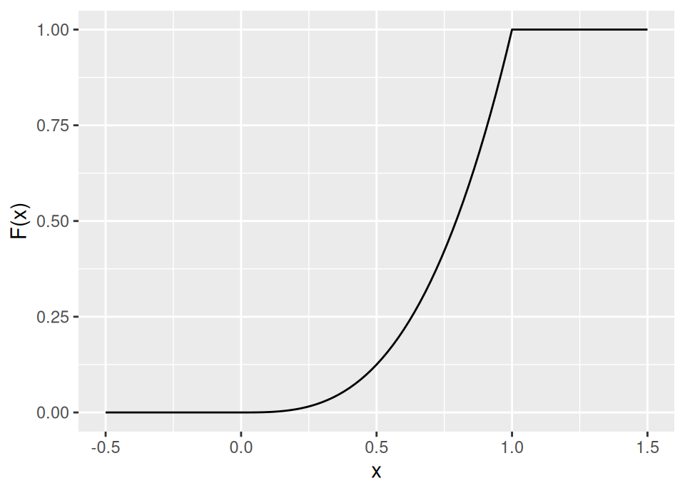
Given the probability density function in the question, we need to find the cdf:

\[F_X(x) = \int_{-\infty}^x \alpha z^{\alpha-1} \, dz = \begin{cases} 0 & \text{if } x < 0 \\ x^\alpha & \text{if } x \in [0,1] \\ 1 & \text{if } x > 1 \end{cases}\]

For example,

Therefore, $F^{-1}(u) = u^{\frac{1}{\alpha}}$.

Hence, we simulate from this probability density function by simulating $U \sim \text{Unif}(0,1)$ and then return $X = u^{\frac{1}{\alpha}}$.

(b)

Let $X$ have probability density function $f_X(x)$ as given in the question, \[\begin{align*} \mu = \int_0^1 x e^{-x} \, dx &= \int_0^1 \frac{1}{f_X(x)} x e^{-x} f_X(x) \, dx \\ &= \int_{\mathbb{R}} \alpha^{-1} x^{-\alpha+1} x e^{-x} f_X(x) \, dx \\ &= \int_{\mathbb{R}} \alpha^{-1} x^{-\alpha+2} e^{-x} f_X(x) \, dx \\ &= \mathbb{E}\left[\alpha^{-1} X^{-\alpha+2} e^{-X}\right] \end{align*}\]

(c)

Simulate $x_1, \dots, x_n$ from the pdf given in the question, perhaps using inverse transform sampling as described in (a)
Calculate \[\hat{\mu}_n = \frac{1}{n} \sum_{i=1}^n \alpha^{-1} x^{-\alpha+2} e^{-x}\]

(d)

As for Q1(d) & Q2(c), we know from lectures that \[\text{Var}\left(\hat{\mu}_n\right) = \mathbb{E}\left[(\hat{\mu}_n - \mu)^2\right] = \frac{\sigma^2}{n}\] However, now \[\sigma^2 = \text{Var}\left(\alpha^{-1} X^{-\alpha+2} e^{-X}\right)\] with $X$ simulated from $f_X(\cdot)$.

We are told $\alpha=2$, so we want:

\[\text{Var}\left(0.5 e^{-X}\right) = \mathbb{E}\left[ \left(0.5 e^{-X}\right)^2 \right] - \mathbb{E}\left[ 0.5 e^{-X} \right]^2\]

We know that Monte Carlo integration is unbiased, so the second term is unchanged in value despite the different problem formulation,

\[\mathbb{E}\left[ 0.5 e^{-X} \right] = 1 - 2e^{-1} \approx 0.2642\]

So we just need:

\[\begin{align*} \mathbb{E}\left[ \left(0.5 e^{-X}\right)^2 \right] &= \int 0.25 e^{-2x} f_X(x) \,dx \\ &= \int_0^1 0.25 e^{-2x} \times 2 x \,dx \\ &= 0.5 \int_0^1 x e^{-2x} \,dx \\ &= 0.5 \left[ -\frac{e^{-2x}}{4} (2x + 1) \right]_0^1 & \text{using hint} \\ &= \frac{1}{8} - \frac{3}{8} e^{-2} \\ &\approx 0.07425 \end{align*}\]

Therefore,

\[\begin{align*} \text{Var}\left(0.5 e^{-X}\right) &= \underbrace{\frac{1}{8} - \frac{3}{8} e^{-2}}_{\mathbb{E}\left[ \left(0.5 e^{-X}\right)^2 \right]} - \underbrace{\left(1 - 2e^{-1}\right)^2}_{\mathbb{E}\left[ 0.5 e^{-X} \right]^2} \\ &= 4 e^{-1} - \frac{35}{8} e^{-2} - \frac{7}{8} \\ &\approx 0.004426 \end{align*}\]

Thus, \[\text{Var}\left(\hat{\mu}_n\right) \approx \frac{0.004426}{n}\]

(e)

The logic is as for Q2(d). So,

\[\frac{0.09078}{0.004426} = 20.51\]

So we would need more than $20\times$ as many simulations from an Exponential to achieve the same accuracy.

\[\frac{0.01101}{0.004426} = 2.49\]

So we would need $2.49\times$ as many simulations from a Uniform to achieve the same accuracy.

Q3

(a)

\[g(x) = \frac{1}{2} \exp(-|x|) \quad \forall\,x \in \mathbb{R}\]

\[\begin{align*} F_g(x) &= \int_{-\infty}^x g(z)\,dz \\ &= \begin{cases} \displaystyle \frac{1}{2} \int_{-\infty}^x \exp(z) \,dz & \text{if }x \le 0 \\ \displaystyle \frac{1}{2} + \frac{1}{2} \int_0^x \exp(-z) \,dz & \text{if }x > 0 \end{cases} \end{align*}\]

The first integral is trivially $e^x$. For the second integral, you can either use a simple symmetry argument, or, to plough through the calculus directly we could use the substitution $u = -z \implies du = -dz$ and limits $u = -0 = 0$ to $u = -x$,

\[\int_0^x \exp(-z) \,dz = -\int_0^{-x} \exp(u) \,du = -e^u \Big|_0^{-x} = 1-e^{-x}\]

Therefore,

\[ F_g(x) = \begin{cases} \displaystyle \frac{e^x}{2} & \text{if }x \le 0 \\ \displaystyle 1 - \frac{e^{-x}}{2} & \text{if }x > 0 \end{cases} \]

The generalised inverse is thus,

\[ F_g^{-1}(u) = \begin{cases} \displaystyle \log(2u) & \text{if }u \le \frac{1}{2} \\ \displaystyle -\log(2-2u) & \text{if }u > \frac{1}{2} \end{cases} \]

Hence, to inverse transform sample a standard Laplace random variable we would generate $U \sim \text{Unif}(0,1)$ and compute $F_g^{-1}(U)$ per above.

(b)

We require $c < \infty$ such that

\[\frac{1}{\sqrt{2 \pi}} \exp\left(-\frac{x^2}{2}\right) \le \frac{c}{2} \exp(-|x|) \quad \forall\ x \in \mathbb{R}\]

Both pdfs are symmetric about zero, so this is equivalent to:

\[\frac{1}{\sqrt{2 \pi}} \exp\left(-\frac{x^2}{2}\right) \le \frac{c}{2} \exp(-x) \quad \forall\ x \in [0,\infty)\]

In other words, we require:

\[c = \sup_{x \in [0,\infty)} \sqrt{\frac{2}{\pi}} \exp\left( -\frac{x^2}{2} + x \right)\]

As $x\to\infty$, the $-x^2/2$ dominates the $+x$, so the exponential term tends to zero and we can see there is no problem in the tail.

Now,

\[\begin{align*} \frac{d}{dx} &= \sqrt{\frac{2}{\pi}} (1-x) \exp\left( -\frac{x^2}{2} + x \right) & \text{Simple chain rule application} \\ \frac{d^2}{dx^2} &= \sqrt{\frac{2}{\pi}} x (x-2) \exp\left( -\frac{x^2}{2} + x \right) & \text{Product and chain rules} \end{align*}\]

By inspection, $d/dx = 0 \iff x = 1$ and at this point $d^2/dx^2 < 0$ confirming this is a maximum. Hence,

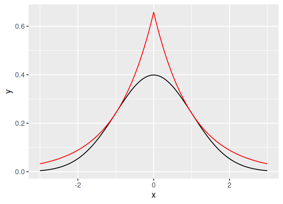
\[c = \sqrt{\frac{2}{\pi}} \exp\left( \frac{1}{2} \right) \approx 1.3155\]

The following graph shows the standard Laplace distribution scaled by $c$ in red, with the standard normal in black, confirming that $c$ satisfies the inequality.

(c)

Set $a \leftarrow \texttt{FALSE}$
While $a$ is $\texttt{FALSE}$,
1. Generate $U_1 \sim \text{Unif}(0,1)$
2. Compute \[X = \begin{cases} \displaystyle \log(2U_1) & \text{if }U_1 \le \frac{1}{2} \\ \displaystyle -\log(2-2U_1) & \text{if }U_1 > \frac{1}{2} \end{cases}\] which generates a proposal from the standard Laplace distribution.
3. Generate $U_2 \sim \text{Unif}(0,1)$
4. If \[U_2 \le \frac{1}{1.3155}\sqrt{\frac{2}{\pi}} \exp\left(-\frac{X^2}{2} + |X|\right)\] then set $a \leftarrow \texttt{TRUE}$
Return $X$ as a sample from $\text{N}(0,1)$.

(d)

By Lemma 5.1, the expected number of iterations of the rejection sampler required to produce a sample is given by $c$, so since here $c\approx1.3155 < 1.521$ we would favour using the standard Laplace distribution as a proposal. The Cauchy proposal would require $(1.521/1.3155 - 1) \times 100\% \approx 15.6\%$ more iterations to produce any given number of standard Normal simulations.

Q4

(a)

By kindergarten rules of probability,

\[\begin{align*} \mathbb{P}(X \le x \given a \le X \le b) &= \frac{\mathbb{P}(a \le X \le b \cap X \le x)}{\mathbb{P}(a \le X \le b)} \\[5pt] &= \frac{\mathbb{P}(a \le X \le b \cap X \le x)}{F(b) - F(a)} \end{align*}\]

Taking the numerator separately,

\[\begin{align*} \mathbb{P}(a \le X \le b \cap X \le x) &= \begin{cases} 0 & \text{if } x < a \\[5pt] \mathbb{P}(a \le X \le x) & \text{if } a \le x \le b \\[5pt] \mathbb{P}(a \le X \le b) & \text{if } x > b \end{cases} \\[10pt] &= \begin{cases} 0 & \text{if } x < a \\[5pt] F(x) - F(a) & \text{if } a \le x \le b \\[5pt] F(b) - F(a) & \text{if } x > b \end{cases} \end{align*}\]

Therefore,

\[ \mathbb{P}(X \le x \given a \le X \le b) = \begin{cases} 0 & \text{if } x < a \\[5pt] \displaystyle \frac{F(x) - F(a)}{F(b)- F(a)} & \text{if } a \le x \le b \\[5pt] 1 & \text{if } x > b \end{cases} \]

(b)

We simply want to find the generalised inverse of the cdf we just derived. So if $U \sim \text{Unif}(0,1)$, then we solve for $X$ in:

\[\begin{align*} U &= \frac{F(X) - F(a)}{F(b)- F(a)} \\[5pt] \implies F(X) &= U \big( F(b)- F(a) \big) + F(a) \\[5pt] \implies X &= F^{-1}\Big( U \big( F(b)- F(a) \big) + F(a) \Big) \end{align*}\]

(c)

For an Exponential distribution, $F(x) = 1-e^{-\lambda x}$ and therefore $F^{-1}(u) = -\lambda^{-1} \log(1-u)$.

Truncating to $X \in [1, \infty) \implies a = 1, b = \infty$, thus $F(a) = 1-e^{-\lambda}, F(b) = 1$ and so the inverse transform sampler is:

\[\begin{align*} X &= F^{-1}\Big( U \big( F(b)- F(a) \big) + F(a) \Big) \\ &= F^{-1}\Big( U \big( 1 - (1-e^{-\lambda}) \big) + (1-e^{-\lambda}) \Big) \\ &= F^{-1}\Big( e^{-\lambda} \big( U - 1 \big) + 1 \Big) \\ &= -\lambda^{-1} \log\Big( 1 - \big( e^{-\lambda} \big( U - 1 \big) + 1 \big) \Big) \\ &= -\lambda^{-1} \log\Big( e^{-\lambda} \big( 1 - U \big) \Big) \\ &= 1 - \lambda^{-1} \log\big( 1 - U \big) \\ \end{align*}\]

(d)

Notice that the inverse transform sampler for the Exponential distribution truncated to $[1, \infty)$ is simply $1 + \big(- \lambda^{-1} \log( 1 - U )\big)$ … in other words, inverse transform sample a standard Exponential and add 1!

This agrees with the well-known memoryless property of the Exponential distribution.

Note: obviously for other distributions it will not be so simple, this is a very special property of Exponential random variables.

Q5

We first find $\mathbb{E}_{f}\left[ h(X) \right]$.

\[\begin{align*} \mathbb{E}_{f}\left[ h(X) \right] &= \int_\mathbb{R} h(x) f(x) \,dx \\ &= \int_0^1 x^2 \,dx \quad\mbox{(NB limits determined by $f$)} \\ &= \left. \frac{x^3}{3} \right|_{x=0}^1 \\ &= \frac{1}{3} \end{align*}\]

\[\begin{align*} \mathbb{E}_{g}\left[ \frac{h(X) f(X)}{g(X)} \right] &= \int_\mathbb{R} \frac{h(x) f(x)}{g(x)} g(x) \,dx \\ &= \int_0^\frac{1}{2} \frac{x^2}{2} \times 2 \,dx \quad\mbox{(NB limits determined by $g$)} \\ &= \int_0^\frac{1}{2} x^2 \,dx \\ &= \frac{1}{24} \end{align*}\]

This is to illustrate the importance of the requirement that $g(\cdot)$ be a pdf such that $g(x) > 0$ whenever $h(x) f(x) \ne 0$ in order for importance sampling to be valid! This condition is clearly violated for the choices of $f(\cdot), g(\cdot)$ and $h(\cdot)$ above.

Q6

(a)

\[\begin{align*} \mathbb{E}_f[X] &= \int_\Omega x f(x) \,dx \\ &= \int_0^1 x (2x) \,dx \\ &= \frac{2}{3} \end{align*}\]

(b)

\[ \hat{\mu}_n = \frac{1}{n} \sum_{i=1}^n x_i \]

\[ \text{Var}(\hat{\mu}_n) = \frac{\text{Var}(h(X))}{n} \] Now $h(X) = X$ here, and \[ \text{Var}(X) = \mathbb{E}[X^2] - \mathbb{E}[X]^2 \] We know $\mathbb{E}[X]$ from part (a), so just need, \[\begin{align*} \mathbb{E}[X^2] &= \int_\Omega x^2 f(x) \,dx \\ &= \int_0^1 x^2 (2x) \,dx \\ &= \frac{1}{2} \end{align*}\] Thus, \[ \text{Var}(X) = \frac{1}{2} - \left(\frac{2}{3}\right)^2 = \frac{1}{18} \approx 0.0556 \] Therefore, \[ \text{Var}(\hat{\mu}_n) = \frac{1}{18n} \]

(c)

\[ \hat{\mu}_n = \frac{1}{n} \sum_{i=1}^n w_i x_i \] where \[ w_i = \frac{f(x_i)}{g(x_i)} = \frac{2x_i}{\alpha x_i^{\alpha-1}} = 2\alpha^{-1}x_i^{2-\alpha} \] Thus, in full, \[ \hat{\mu}_n = \frac{1}{n} \sum_{i=1}^n 2\alpha^{-1}x_i^{3-\alpha} \]

Next, for the variance, we know from lectures, \[\begin{align*} \mathrm{Var}(\hat\mu_n) = \frac{\sigma_{g}^2}{n} \ \text{ where } \ \sigma_{g}^2 = \int_{\tilde{\Omega}} \frac{\left( h(x) f(x) - \mu g(x) \right)^2}{g(x)}\,dx, \end{align*}\] and recall that here $h(x)=x$ and from (a) $\mu = \frac{2}{3}$. Thus, (not necessary to show all these small steps, but providing full detail for solutions …) \[\begin{align*} \sigma_{g}^2 &= \int_{\tilde{\Omega}} \frac{\left( h(x) f(x) - \mu g(x) \right)^2}{g(x)}\,dx \\ &= \int_0^1 \frac{\left( x (2x) - \frac{2}{3} \alpha x^{\alpha-1} \right)^2}{\alpha x^{\alpha-1}} \,dx \\ &= \int_0^1 \frac{4}{9} \alpha^{-1} x^{1-\alpha} \left( 3x^2 - \alpha x^{\alpha-1} \right)^2 \,dx \\ &= \int_0^1 \frac{4}{9} \alpha^{-1} x^{1-\alpha} \left( 9x^4 - 6 \alpha x^{\alpha+1} + \alpha^2 x^{2\alpha-2} \right) \,dx \\ &= \int_0^1 \frac{4 \alpha x^{\alpha-1}}{9} + \frac{4 x^{5-\alpha}}{\alpha} - \frac{8x^2}{3} \,dx \\ &= \left. \frac{4 x^{\alpha}}{9} + \frac{4 x^{6-\alpha}}{\alpha (6-\alpha)} - \frac{8x^3}{9} \right|_{x=0}^1 \quad \mbox{assuming } 0 < \alpha < 6 \\ &= \frac{4}{\alpha (6-\alpha)} - \frac{4}{9} \end{align*}\]

Note: the distribution $g$ only required $\alpha > 0$, but this variance calculation now only holds for $\alpha \in (0,6)$. This arose because the $x=0$ end of the integral is indeterminate for the term $x^{6-\alpha}$ if $\alpha > 6$ and $\frac{1}{6-\alpha}$ is indeterminate if $\alpha=6$.

\[ \implies \mathrm{Var}(\hat\mu_n) = \frac{4}{n \alpha (6-\alpha)} - \frac{4}{9n}, \quad \alpha \in (0,6) \]

(d)

We are interested in values of $\alpha$ for which it is true that,

\[\begin{align*} \frac{4}{\alpha (6-\alpha)} - \frac{4}{9} &< \frac{1}{18} \\ \implies \frac{4}{\alpha (6-\alpha)} &< \frac{1}{2} \\ \end{align*}\]

Now, the variance only holds for $\alpha \in (0,6)$, so $\alpha (6-\alpha)$ is always positive. Thus we may rearrange without fear of flipping the inequality. So, \[\begin{align*} \implies 8 &< \alpha (6-\alpha) \quad \mbox{for } \alpha \in (0,6) \\ \implies 0 &< (2-\alpha) (\alpha-4) \quad \mbox{for } \alpha \in (0,6) \end{align*}\]

Now $(2-\alpha) (\alpha-4)$ is quadratic in $\alpha$ with negative coefficient on the square term, so this inequality holds only between the roots.

Thus, the variance of importance sampling is smaller than standard Monte Carlo when using proposal $g(\cdot \,|\, \alpha)$ for any $\alpha \in (2,4)$.

(e)

\[ g_{\mathrm{opt}}(x) = \frac{ |h(x)| f(x) }{ \int_\Omega |h(x)| f(x)\,dx } \]

Recall, here $h(x)=x$, so

\[ g_{\mathrm{opt}}(x) = \frac{ |x| 2x }{ \int_0^1 |x| 2x\,dx } \]

But, since $f(x)$ is only non-zero on $[0,1]$, the absolute value can be dropped and we find the optimal proposal is simply:

\[ g_{\mathrm{opt}}(x) = 3 x^2 \]

Yes, this does belong to the family $g(\cdot \,|\, \alpha)$, corresponding to the case $\alpha=3$.

Using part (c), this tells us the variance when using this estimator is:

\[ \mathrm{Var}(\hat\mu_n) = \frac{4}{n \alpha (6-\alpha)} - \frac{4}{9n} = \frac{4}{n 3 (6-3)} - \frac{4}{9n} = 0 \]

Zero variance!?! Note, this implies that if I take even one simulation from $g(\cdot \,|\, \alpha=3)$ that the estimator $\hat\mu_1$ will be exactly correct … does this make sense? Yes! Because also from part (c), we have,

\[\begin{align*} \hat{\mu}_n &= \frac{1}{n} \sum_{i=1}^n 2\alpha^{-1}x_i^{3-\alpha} \\ &= \frac{1}{n} \sum_{i=1}^n 2\times3^{-1}x_i^{3-3} \\ &= \frac{1}{n} \sum_{i=1}^n \frac{2}{3} \\ &= \frac{2}{3} \equiv \mu \end{align*}\]

Note: this is obviously a situation we would never be in when using importance sampling for a real problem which actually required it! Usually, the optimal proposal is inaccessible to us, because to get it we would need to be able to do the original integral anyway. The point here is to highlight that if we can get close to approximating the optimal proposal, then clearly we can dramatically reduce the variance of our estimator.

Q7

Here, the weight for a sample $x_i$ from $g$ will be:

\[ w_i = \frac{f(x_i)}{g(x_i)} = \frac{\lambda e^{-\lambda x_i}}{\eta e^{-\eta x_i}} = \frac{\lambda}{\eta} e^{-(\lambda-\eta) x_i} \]

Now $x_i \in [0, \infty)$ since the Exponential distribution is on the half real line. Notice the term $e^{-(\lambda-\eta) x_i}$ … in order for the weights to be bounded for all possible $x_i$, we need $\lambda-\eta \ge 0$. Thus, the weights are only bounded for $\eta \le \lambda$.