WS 2b: Base R data exploration
🧑💻 Make sure to finish previous work sheets before continuing with this one! It might be tempting to skip some stuff if you’re behind, but you may just end up progressively more lost … we will happily answer questions from any work sheet each week 😃
5.4 Diamonds 💎 data
You have now seen some data comes built into R, or an add-on package to R, because it is useful for learning or experimenting. We will use one such data set which is of a decent size so that it becomes clear you can’t just sift through many data sets, you really do need the tools we’ve learned in the lecture practicals to answer interesting questions.
Exercise 5.33 We will install, load and read about the diamonds data:
- Install the package
ggplot2from CRAN - Load the
diamondsdata from theggplot2package - Look at the help file for this data to learn a little about what variables were collected.
Click for solution
We will use this data to do a series of quick-fire exercises, then a few that you may need a little longer to figure out.
You should not need to write lots of code to answer these questions if you are using the methods from the course so far.
Exercise 5.34 How many observations and how many variables are there in the data?
Click for solution
[1] 53940[1] 10[1] 53940 10Exercise 5.35 How many factor type variables are there?
Click for solution
Remember from lectures that factors are categorical data types, which are handled quite differently from numeric data.
There are a few ways to answer this … perhaps the simplest is to use our good friend str() to examine the structure of the data set:
tibble [53,940 × 10] (S3: tbl_df/tbl/data.frame)
 $ carat  : num [1:53940] 0.23 0.21 0.23 0.29 0.31 0.24 0.24 0.26 0.22 0.23 ...
 $ cut    : Ord.factor w/ 5 levels "Fair"<"Good"<..: 5 4 2 4 2 3 3 3 1 3 ...
 $ color  : Ord.factor w/ 7 levels "D"<"E"<"F"<"G"<..: 2 2 2 6 7 7 6 5 2 5 ...
 $ clarity: Ord.factor w/ 8 levels "I1"<"SI2"<"SI1"<..: 2 3 5 4 2 6 7 3 4 5 ...
 $ depth  : num [1:53940] 61.5 59.8 56.9 62.4 63.3 62.8 62.3 61.9 65.1 59.4 ...
 $ table  : num [1:53940] 55 61 65 58 58 57 57 55 61 61 ...
 $ price  : int [1:53940] 326 326 327 334 335 336 336 337 337 338 ...
 $ x      : num [1:53940] 3.95 3.89 4.05 4.2 4.34 3.94 3.95 4.07 3.87 4 ...
 $ y      : num [1:53940] 3.98 3.84 4.07 4.23 4.35 3.96 3.98 4.11 3.78 4.05 ...
$ z : num [1:53940] 2.43 2.31 2.31 2.63 2.75 2.48 2.47 2.53 2.49 2.39 ...Exercise 5.36 The cut variable is a factor, but is it in a useful order?
Remember the forcats package from the lecture helps us handle factors.
- Load the
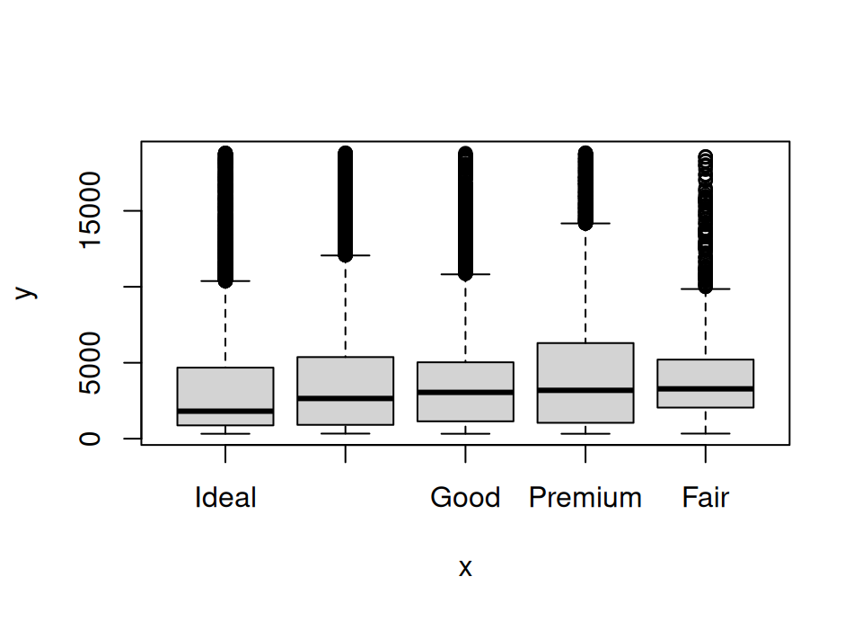
forcatslibrary (you may need to install it first). - Plot
price(y-axis) againstcut(x-axis) using just the baseplot()function. Note the order of the categories on the x-axis. - Use
fct_reorderto reorder thecutfactor based on the medianpriceand plot it again.

 Note: you may need to increase the size of your plotting area to properly see the x-axis labels.
Exercise 5.37 Print just the first few observations in the data.
Click for solution
# A tibble: 6 × 11
  carat cut      color clarity depth table price     x     y     z cut.reordered
  <dbl> <ord>    <ord> <ord>   <dbl> <dbl> <int> <dbl> <dbl> <dbl> <ord>
1  0.23 Ideal    E     SI2      61.5    55   326  3.95  3.98  2.43 Ideal
2  0.21 Premium  E     SI1      59.8    61   326  3.89  3.84  2.31 Premium
3  0.23 Good     E     VS1      56.9    65   327  4.05  4.07  2.31 Good
4  0.29 Premium  I     VS2      62.4    58   334  4.2   4.23  2.63 Premium
5  0.31 Good     J     SI2      63.3    58   335  4.34  4.35  2.75 Good
6  0.24 Very Go… J     VVS2     62.8    57   336  3.94  3.96  2.48 Very Good
# Or, the above shows 6 rows by default, add a number to change how many to
# peek at, eg
head(diamonds, 10)# A tibble: 10 × 11
carat cut color clarity depth table price x y z cut.reordered
<dbl> <ord> <ord> <ord> <dbl> <dbl> <int> <dbl> <dbl> <dbl> <ord>
1 0.23 Ideal E SI2 61.5 55 326 3.95 3.98 2.43 Ideal
2 0.21 Premium E SI1 59.8 61 326 3.89 3.84 2.31 Premium
3 0.23 Good E VS1 56.9 65 327 4.05 4.07 2.31 Good
4 0.29 Premium I VS2 62.4 58 334 4.2 4.23 2.63 Premium
5 0.31 Good J SI2 63.3 58 335 4.34 4.35 2.75 Good
6 0.24 Very G… J VVS2 62.8 57 336 3.94 3.96 2.48 Very Good
7 0.24 Very G… I VVS1 62.3 57 336 3.95 3.98 2.47 Very Good
8 0.26 Very G… H SI1 61.9 55 337 4.07 4.11 2.53 Very Good
9 0.22 Fair E VS2 65.1 61 337 3.87 3.78 2.49 Fair
10 0.23 Very G… H VS1 59.4 61 338 4 4.05 2.39 Very Good Exercise 5.38 What are the summary statistics (eg min/max, mean, median, counts, …) for each variable?
Click for solution
     carat               cut        color        clarity          depth
 Min.   :0.2000   Fair     : 1610   D: 6775   SI1    :13065   Min.   :43.00
 1st Qu.:0.4000   Good     : 4906   E: 9797   VS2    :12258   1st Qu.:61.00
 Median :0.7000   Very Good:12082   F: 9542   SI2    : 9194   Median :61.80
 Mean   :0.7979   Premium  :13791   G:11292   VS1    : 8171   Mean   :61.75
 3rd Qu.:1.0400   Ideal    :21551   H: 8304   VVS2   : 5066   3rd Qu.:62.50
 Max.   :5.0100                     I: 5422   VVS1   : 3655   Max.   :79.00
                                    J: 2808   (Other): 2531
     table           price             x                y
 Min.   :43.00   Min.   :  326   Min.   : 0.000   Min.   : 0.000
 1st Qu.:56.00   1st Qu.:  950   1st Qu.: 4.710   1st Qu.: 4.720
 Median :57.00   Median : 2401   Median : 5.700   Median : 5.710
 Mean   :57.46   Mean   : 3933   Mean   : 5.731   Mean   : 5.735
 3rd Qu.:59.00   3rd Qu.: 5324   3rd Qu.: 6.540   3rd Qu.: 6.540
 Max.   :95.00   Max.   :18823   Max.   :10.740   Max.   :58.900

       z            cut.reordered
 Min.   : 0.000   Ideal    :21551
 1st Qu.: 2.910   Very Good:12082
 Median : 3.530   Good     : 4906
 Mean   : 3.539   Premium  :13791
 3rd Qu.: 4.040   Fair     : 1610
 Max.   :31.800
summary() has been sensible and just given us counts for the factor variables.
Exercise 5.39 A key part of exploring a new dataset is checking for missing data.
Use the any() and is.na() functions to check if the diamonds dataset contains any missing values.
Exercise 5.40 Find the total value of all ideal cut diamonds, with colour code D and with depth percentage of 60 or less.
Is that total value greater or less than $200,000?
Click for solution
## SOLUTION

sum(diamonds[diamonds$cut == "Ideal" & diamonds$color == "D" & diamonds$depth <= 60,"price"])
[1] 196479Exercise 5.41 Create a new variable named ppc in the diamonds data frame which contains the price per carat of each diamond. Then compute the overall median price per carat.
Click for solution
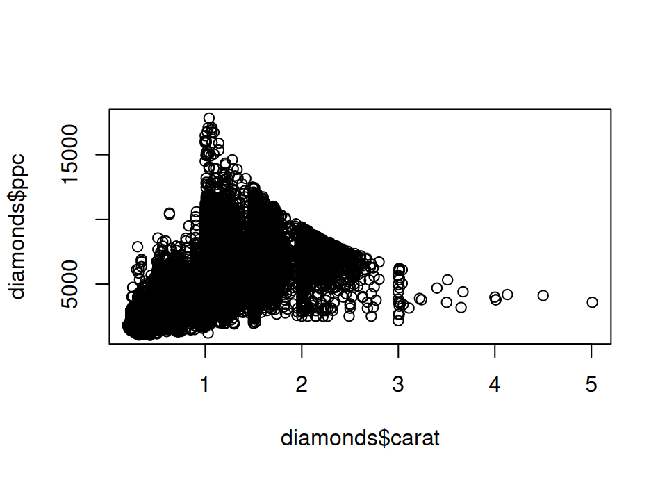
[1] 3495.198Exercise 5.42 Plot a simple scatterplot of caret on the x-axis and ppc on the y-axis. (Note: this is a bigger dataset, so this plot might take a few seconds to display after you run the function)
We can add horizontal or vertical lines to our plots with the abline() function. For example, if you run abline(v = 1) it will add a vertical line which crosses the x-axis at 1. If you run abline(h = 1000) it will add a horizontal line which crosses the y-axis at 1000.
Exercise 5.43 We will add some visual guides to help us:
- add a horizontal line to your plot at the mean price per carat
- add vertical lines at carat equals 1, 2, 3, 4 and 5
- Using these visual guides, roughly what range of carats seem to attract the highest price per carat?
Click for solution
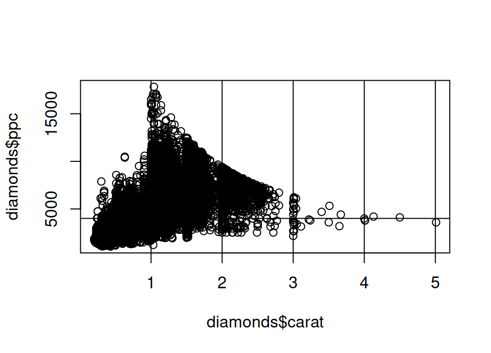
- It looks like many diamonds between 1 and 2 carats attract a large premium in the price you pay per carat.
- Indeed, there is something of a cliff edge effect at the 1 carat value. Can you speculate why?
- This is somewhat, but less, in evidence between 2 and 3 carats: in this case the spread above the mean is not so exaggerated compared to the spread below the mean.
- Across all carat levels there is a lot of spread though, so within all ranges there are some diamonds which are very average in the price per carat.
Exercise 5.44 Create two new data frames. Both should contain only the diamonds whose carat is between 1 and 2 and:
- the first should have
ppcexceeding 10000 - the second should have
ppcless than or equal to 10000
Using these data frames, provide counts of the clarity variable for each data frame. Is there a clear difference?
Click for solution
## SOLUTION

high.ppc <- diamonds[diamonds$ppc>10000 & diamonds$carat >= 1 & diamonds$carat < 2,]
normal.ppc <- diamonds[diamonds$ppc<=10000 & diamonds$carat >= 1 & diamonds$carat < 2,]

table(high.ppc$clarity)
  I1  SI2  SI1  VS2  VS1 VVS2 VVS1   IF
   0    0    0   77  115  167  144  110
  I1  SI2  SI1  VS2  VS1 VVS2 VVS1   IF
 415 4220 4511 3641 2179  901  286  140
According to the documentation we saw at the start of the work sheet, clarity is a measurement of how clear the diamond is (I1 (worst), SI2, SI1, VS2, VS1, VVS2, VVS1, IF (best))
Clearly the high price per carat diamonds contain only diamonds of clarity VS2 or better. The vast majority of normal price per carat diamonds are of clarity VS1 or worse. So clarity is perhaps one factor contributing to the excessive price per carat of diamonds in this carat range.Exercise 5.45 What is the price, number of carats, cut and clarity of the most expensive diamond in the data?
Click for solution
## SOLUTION

pricy <- diamonds[order(diamonds$price, decreasing = TRUE)[1], c("price", "carat", "cut", "clarity")]
pricy
# A tibble: 1 × 4
price carat cut clarity
<int> <dbl> <ord> <ord>
1 18823 2.29 Premium VS2 To help understand the above, break it down:
order(diamonds$price)provides the row numbers from lowest to highest priceorder(diamonds$price, decreasing = TRUE)switches this to highest to lowest priceorder(diamonds$price, decreasing = TRUE)[1]gets just the first element, in other words the row number of the highest priced diamond- The above is passed as the row value in the
[ , ]and the vector of column names is provided in the column values.
Exercise 5.46 Are there any diamonds in the data which have more carats, superior cut and superior clarity than the most expensive diamond? What is the biggest saving you could make if you just wanted to improve on these characteristics versus the most expensive diamond?
Click for solution
## SOLUTION

# Yes, the following has more than zero rows, so there are cheaper diamonds
# which are better on all those characteristics
improve <- diamonds[diamonds$carat > pricy$carat & diamonds$cut > pricy$cut & diamonds$clarity > pricy$clarity,]
improve
# A tibble: 4 × 12
carat cut color clarity depth table price x y z cut.reordered
<dbl> <ord> <ord> <ord> <dbl> <dbl> <int> <dbl> <dbl> <dbl> <ord>
1 2.59 Ideal J VS1 61.7 56 16465 8.83 8.77 5.43 Ideal
2 2.39 Ideal J VS1 62.1 57 17365 8.53 8.57 5.31 Ideal
3 2.36 Ideal J VS1 61.6 57 17829 8.6 8.55 5.28 Ideal
4 2.32 Ideal J VS1 62.5 54.5 17891 8.44 8.47 5.28 Ideal
# ℹ 1 more variable: ppc <dbl>[1] 2358🏁🏁 Done, end of work sheet! 🏁🏁