Using Couplings in Monte Carlo
Supervisor: Prof. L.J.M. Aslett
Simulation is a vital tool for statisticians. If you took ‘Data Science and Statistical Computing II’ last year, you’ll be familiar with simulation methods like inverse transform sampling, rejection sampling, and importance sampling, and their applications in hypothesis testing, bootstrapping, and integration. Those taking ‘Bayesian Computation and Modelling III’ this year will delve into more advanced techniques such as Markov chain Monte Carlo (MCMC) and Sequential Monte Carlo (SMC), in the context of Bayesian inference.
While simpler methods like inverse transform and rejection sampling have the advantage of producing exact simulations from a probability distribution, there are many distributions for which they cannot be used. More advanced techniques overcome these limitations, but often rely on asymptotic theory, meaning the simulations are only distributed correctly in the limit of infinite samples. In practice, this can lead to uncertainty about whether simulations are truly unbiased or if some bias is present due to finite sample sizes.
Given its central importance, simulation is a very active area of research. One technique that you will not have studied in lectures is so-called ‘coupling’ methods. Coupling of random variables aims to simulate from a joint distribution, \( (X, Y) \), in such a way that the marginal distributions follow some desired choices, say, \( X \sim \pi_1, Y \sim \pi_2 \). The key is that the joint distribution is specifically constructed to possess an interesting structure that can be exploited. For instance, we might aim for a high probability that \( Y = g(X) \) for some function \( g \), while still preserving the specified marginal distributions \( \pi_1 \) and \( \pi_2 \).
For example, the following figure shows a coupling where the marginals are uniform, yet with high probability \( Y = 2X \).
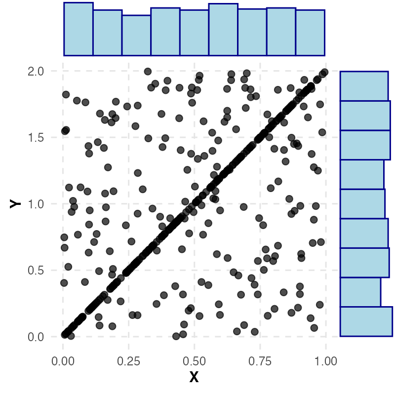
A coupling which has marginals \( X \sim \text{Unif}(0,1) \) and \( Y \sim \text{Unif}(0,2) \), where around half the samples satisfy \( Y = 2X \).
It might not be immediately clear how coupling methods improve statistical simulations. That’s precisely what this project aims to explore! These coupling constructions have a rich history in various Monte Carlo methods, including early applications in perfect simulation methods (Propp and Wilson, 1996) and Markov chain convergence diagnostics (Johnson, 1996). More recently, there has been renewed interest, highlighted by significant work in unbiasing MCMC (Jacob et al, 2020).
Summary
In this project, you will start out learning coupling concepts and getting an understanding of MCMC, including why biases can occur in finite-length chains. From there, you’ll have the flexibility to explore different avenues, focusing on how coupling methods can be applied to MCMC or other Monte Carlo techniques.
Modules
Essential prior modules are Data Science and Statistical Computing II, Statistical Inference II, and Probability I. The project will involve coding up various coupling and Monte Carlo algorithms in R.
It is strongly advised to take Bayesian Computation and Modelling III whilst doing this project, as most of the ways to use couplings that we will look at involve MCMC, so it is very synergistic with that module.
References
Jacob, P.E., O’Leary, J. and Atchadé, Y.F. (2020) “Unbiased Markov Chain Monte Carlo Methods with Couplings,” Journal of the Royal Statistical Society Series B: Statistical Methodology, 82(3), pp. 543–600. doi:10.1111/rssb.12336.
Johnson, V.E. (1996) “Studying Convergence of Markov Chain Monte Carlo Algorithms Using Coupled Sample Paths,” Journal of the American Statistical Association, 91(433), pp. 154–166. doi:10.1080/01621459.1996.10476672.
Propp, J.G. and Wilson, D.B. (1996) “Exact sampling with coupled Markov chains and applications to statistical mechanics,” Random Structures and Algorithms, 9(1–2), pp. 223–252. doi:10.1002/(sici)1098-2418(199608/09)9:1/2<223::aid-rsa14>3.0.co;2-o.
