class: center, middle, inverse, title-slide .title[ # Data Science and Statistical Modelling ] .subtitle[ ## Practical Lecture 6<br>Dynamic Documents ] .author[ ### Prof. Louis Aslett ] .institute[ ### Durham University ] .date[ ### 3 February 2026 ] --- <style type="text/css"> .remark-slide-content { font-size: 125% !important; } .smaller .remark-code { /*Change made here*/ font-size: 80% !important; } </style> ## Dynamic documents? **What?** - Combines report writing/slides/etc *and* code *and* data source in one file. - Change input data and the document will dynamically update. - Single source for multiple output formats (HTML, PDF, Word) - Single language for multiple output types (presentations, reports, books, papers, ...) -- **Why?** A major challenge for using data in industry, commercial and research settings is that reporting can become separated from the data itself, leading to problems in tracing how a particular graphic, statistic, etc was produced. - Harms reproducibility - Slows down making changes to graphics/analysis - Updating with new data slow - Error prone if process by which document generated is obfuscated -- RMarkdown allows us to mix content and code in a *plain text* format (no WYSIWYG). --- background-image: url(i/word_meme.jpg) background-size: contain class: center, bottom, inverse --- class: inverse ## Getting the packages ``` r install.packages("rmarkdown") install.packages("tinytex") ``` `tinytex` includes a miniture LaTeX distribution so that you can compile to PDFs! RStudio already includes the packages needed for Quarto, so you won't need to separately install those if you're using Codespaces (but you still need `tinytex` for PDF). If you're not on Codespaces, you may need to ask for help in the practical help session if you want to test Quarto. --- ## RMarkdown - Simple plain text format - Separate presentational style from content - Simplified formatting commands - Embedded code - Include LaTeX for mathematical content  --- ## Document preamble Section enclosed between two lines of `---` at the top is the "document preamble". Specifies various options for the document, including: - `title:` the document title - `author:` (optional) author's name - `date:` (optional) date for the document - `output:` a tree like structure for setting options of different output formats (HTML/PDF/Word) <img src="i/rmarkdown_opts.png" alt="" width="60%" style="display: block; margin: auto;" /> --- ## Simple formatting Styles: - `*italic text*` - *italic text* - `**bold text**` - **bold text** - `~~strikeout text~~` - ~~strikeout text~~ Sections: - `# Section heading` - 1. Section heading - `## Sub-section heading` - 1.1 Sub-section heading - `### Sub-sub-section heading` - 1.1.1 Sub-sub-section heading Misc: - `[Prof. Aslett's homepage](https://www.louisaslett.com/)` - [Prof. Aslett's homepage](https://www.louisaslett.com/) --- ## Lists .pull-left[ - First item - Second item - First sub-item - Second sub-item - Third item ] .pull-right[ ``` r - First item - Second item - First sub-item - Second sub-item - Third item ``` ] .pull-left[ 1. First item 1. Second item i. First sub-item ii. Second sub-item 1. Third item ] .pull-right[ ``` r 1. First item 1. Second item i. First sub-item i. Second sub-item 1. Third item ``` ] **Note:** 4 spaces needed to create the indent **Note:** Don't need to increment the numbering manually --- ## Including R code and output (inline) R can be included inline in text very easily. eg: ``` r `r 1+1` ``` will substitute the value 2 in that place. To show the code in a code font, but not execute, don't include the "r". eg: ``` r `1+1` ``` will make the text look like this `1+1`. --- ## Including R code and output (chunks) I Use the triple-backtick fence, specifying the language to be R. <code> ```{r} <br> x <- rnorm(10, 3) <br> mean(x) <br> ``` </code> Prints both the code (nicely formatted) and the result of executing that code: ``` r x <- rnorm(10, 3) mean(x) ``` ``` [1] 2.837827 ``` --- ## Including R code and output (chunks) II Various options change the behaviour, including: - `echo=FALSE` to suppress printing the code (just show the output) - `eval=FALSE` to show the code, but not run it Obviously using both together is ... largely pointless! -- Plots can be included by simply calling the plotting command. - `fig.width` and `fig.height` take numeric options to specify size - `out.width` and `out.height` allow character options (eg "25%") to proportionately scale. --- <code> ```{r,echo=FALSE} <br> hist(x, main="Histogram of 100 Normal(mean=3, sd=1)") <br> ``` </code> 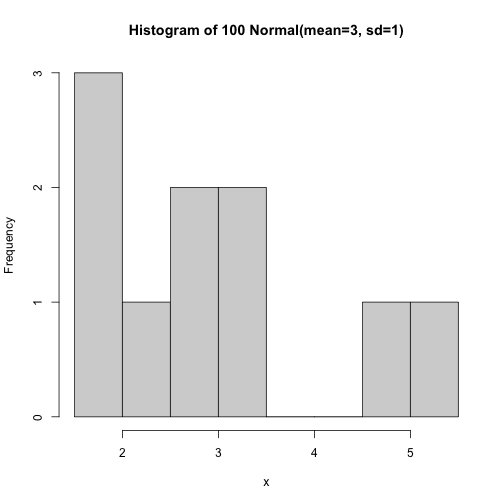<!-- --> --- ## Tables ``` html | Col1 | Col2 | Col3 | Col4 | Col5 | |------|------|-----:|------|:----:| | a | 1 | x | `a` | x | | b | 2 | y | `b` | y | ``` | Col1 | Col2 | Col3 | Col4 | Col5 | |------|------|-----:|------|:----:| | a | 1 | x | `a` | x | | b | 2 | y | `b` | y | -- See also the great package `gt` [https://gt.rstudio.com](https://gt.rstudio.com) --- ## Maths You can write LaTeX inside a pair of dollar symbols, eg: `$\alpha+\beta$` renders `\(\alpha+\beta\)` You can use the display style with double dollar signs: ``` $$\bar{X}=\frac{1}{n}\sum_{i=1}^nX_i$$ ``` `$$\bar{X}=\frac{1}{n}\sum_{i=1}^nX_i$$` -- ``` \begin{align*} asd &= asd \\ &= asd \end{align*} ``` `\begin{align*} e^{i \pi} &= \cos \pi + i \sin \pi \\ &= -1 \end{align*}` --- ## Presentations Exactly the same source can support generating presentations rather than documents! Main difference: `##` triggers a new slide. --- ## Resources See also: - R Markdown cheat sheet - [https://github.com/rstudio/cheatsheets/raw/main/rmarkdown.pdf](https://github.com/rstudio/cheatsheets/raw/main/rmarkdown.pdf) - R Markdown website has good gallery of examples: - [https://rmarkdown.rstudio.com](https://rmarkdown.rstudio.com) - R Markdown books: - The Definitive Guide [https://bookdown.org/yihui/rmarkdown/](https://bookdown.org/yihui/rmarkdown/) - Cookbook [https://bookdown.org/yihui/rmarkdown-cookbook/](https://bookdown.org/yihui/rmarkdown-cookbook/)